(This post originated from my talk for the WiMLDS x Fintech meetup, hosted by Affirm.)

Many of you have likely watched, or at least heard about, the games played in 2016 between AlphaGo and professional Go player Lee Sedol. Lee holds the highest rank of nine dan and has won many world championships. He is unquestionably among the best Go players in the world, yet he lost 1-4 in that series against AlphaGo. Prior to this, Go was widely considered intractable for computers to master because its simple rules generate an exponential number of possible board-position variations, far more than in chess. This event clearly made 2016 a landmark year for AI. In the wake of AlphaGo, attention to AI progress increased substantially.

At the same time, many companies are investing in expanding the boundaries of AI applications that have the potential to change, or even revolutionize, how we live. Common examples include self-driving cars, chatbots, home assistant devices, and many others. One of the key ingredients behind the progress of recent years is deep learning.

Why Does Deep Learning Work Now?

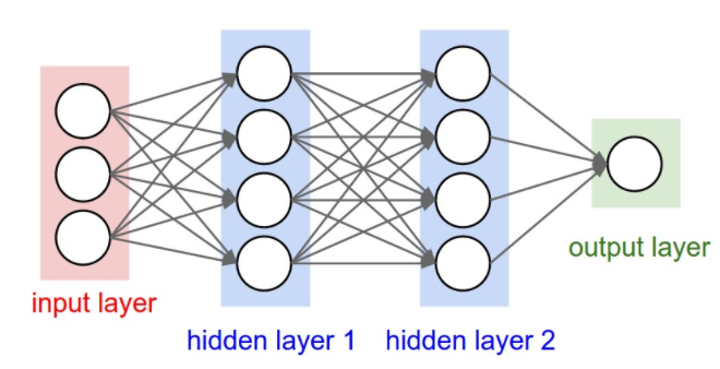
In simple terms, deep learning models are large, deep artificial neural networks. A neural network (“NN”) can be represented as a directed acyclic graph: the input layer receives signal vectors, and one or more hidden layers transform the output of the preceding layer. The earliest idea of a neural network dates back more than half a century. So why does it work now, and why has it become a major topic so suddenly?

The answer is surprisingly straightforward:

• We have far more data.
• We have much more powerful computers.

A large, deep neural network includes many more layers and many more nodes per layer, which leads to exponentially more parameters to tune. Without sufficient data, we cannot learn those parameters effectively. Without powerful computers, training becomes too slow and inadequate.

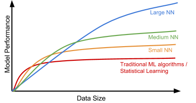
The following plot, proposed by Andrew Ng in his talk “Nuts and Bolts of Applying Deep Learning,” illustrates the relationship between data scale and model performance. With small datasets, traditional algorithms (Regression, Random Forests, SVM, GBM, etc.) or statistical learning can perform extremely well. However, as the data scale grows dramatically, large NNs begin to outperform the alternatives. One reason is that, relative to traditional ML models, neural networks have many more parameters and can learn complex nonlinear patterns. As a result, we often expect the model to discover the most useful features on its own, without extensive expert-driven manual feature engineering.

Deep Learning Models

Next, we will review several classical deep learning models.

Convolutional Neural Network

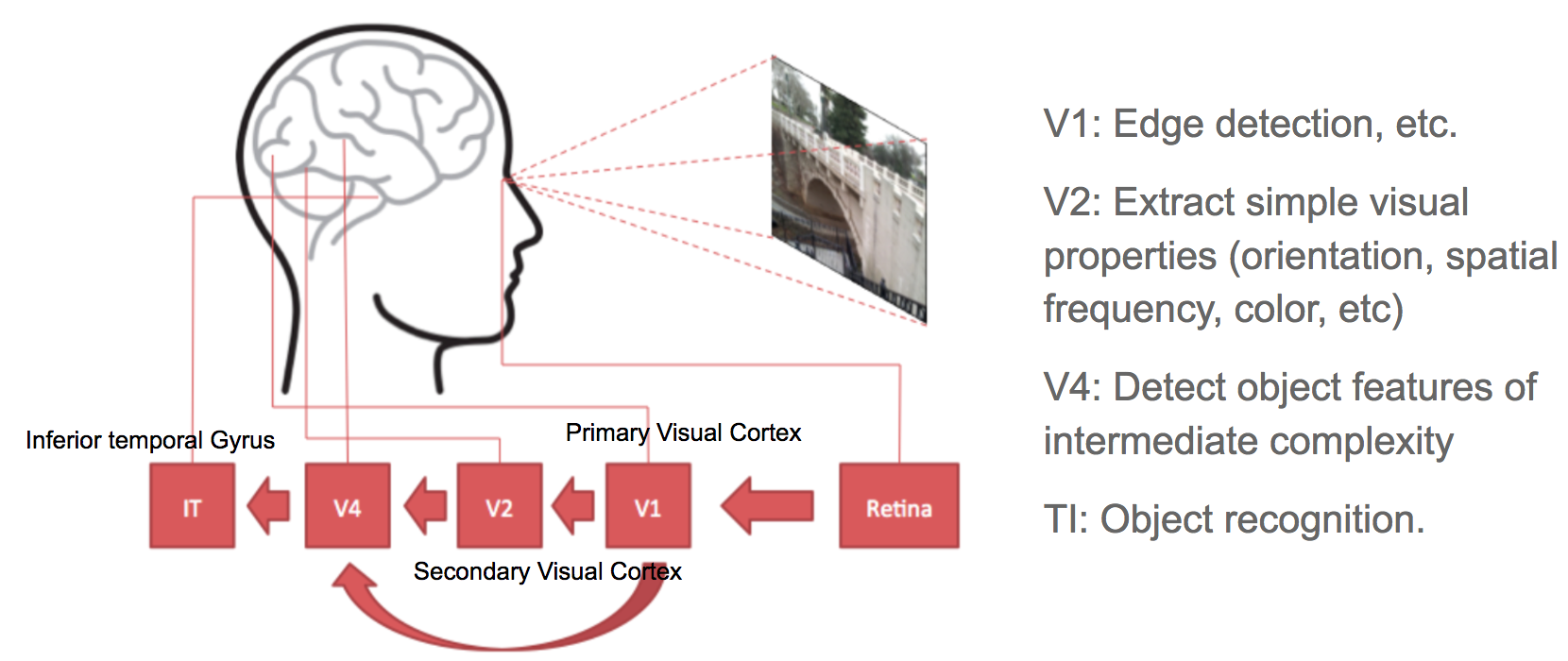
Convolutional neural networks, abbreviated “CNN,” are a type of feed-forward artificial neural network whose connectivity pattern is inspired by the organization of the visual cortex. The primary visual cortex (V1) performs edge detection from raw visual input received from the retina. The secondary visual cortex (V2), also called the prestriate cortex, receives edge features from V1 and extracts basic visual properties such as orientation, spatial frequency, and color. The visual area V4 handles more complex object attributes. These processed features then flow into the final logic unit, the inferior temporal gyrus (IT), for object recognition. The shortcut pathway between V1 and V4 inspired a special CNN architecture with connections between non-adjacent layers: the Residual Net (He, et al. 2016), which includes “Residual Blocks” that allow an input from one layer to be passed to a component two layers later.

Convolution is a mathematical term that, in this context, refers to an operation between two matrices. A convolutional layer uses a fixed, small matrix, also known as a kernel or filter. As the kernel slides (convolves) across the matrix representation of the input image, it computes element-wise multiplications between kernel values and the corresponding values in the original image. Specially designed kernels can process images for common tasks such as blurring, sharpening, and edge detection, both quickly and efficiently.

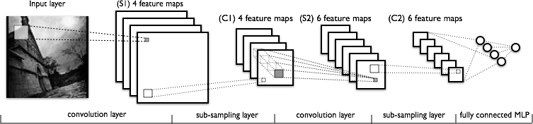
Convolutional and pooling layers (or “sub-sampling,” as labeled in Fig. 4) function analogously to the V1, V2, and V4 units of the visual cortex by performing feature extraction. The object-recognition reasoning occurs later, in the fully-connected layers that consume these extracted features.

Recurrent Neural Network

A sequence model is typically designed to transform an input sequence into an output sequence that resides in a different domain. Recurrent neural networks, abbreviated “RNN,” are well suited to this setting and have delivered major improvements in tasks such as handwriting recognition, speech recognition, and machine translation (Sutskever et al. 2011, Liwicki et al. 2007).

An RNN is inherently capable of processing long sequential data and addressing tasks where context evolves over time. The model processes a single element of the sequence at each time step. After computing, the updated unit state is passed to the next time step to support computation for the next element. For example, imagine an RNN that reads all Wikipedia articles character by character, and then predicts the next words given the preceding context.

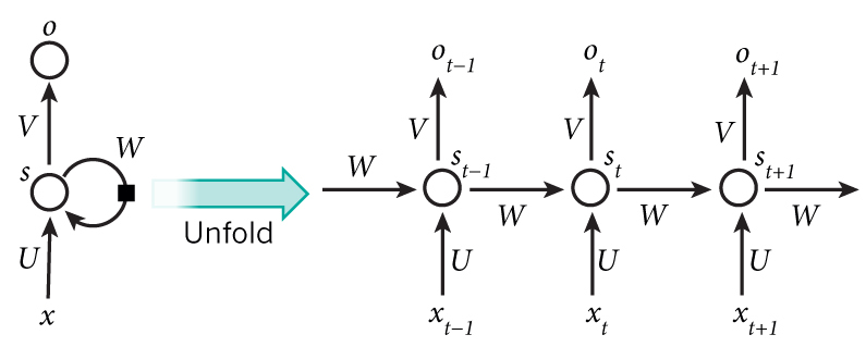
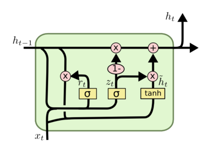
However, simple perceptron neurons that linearly combine the current input element with the previous unit state can easily fail to preserve long-term dependencies. Consider a sentence that begins with “Alice is working at …” and then, after an entire paragraph, the next sentence should begin correctly with “She” or “He.” If the model has forgotten the name “Alice,” it cannot make the correct choice. To address this limitation, researchers introduced a specialized neuron with a substantially more complex internal structure for maintaining long-term context, called the “Long-short term memory (LSTM)” cell. It can learn how long to retain old information, when to forget it, when to incorporate new data, and how to combine existing memory with new input. This introduction is exceptionally well written, and I recommend it to anyone interested in LSTMs. It has also been officially promoted in the Tensorflow documentation ;-)

To demonstrate the capabilities of RNNs, Andrej Karpathy built a character-based language model using an RNN with LSTM cells. Without any preexisting knowledge of English vocabulary, the model learned relationships between characters to form words, and then relationships between words to form sentences. It achieved respectable performance even without a massive training dataset.

RNN: Sequence-to-Sequence Model

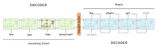
The sequence-to-sequence model extends the RNN. Its application area is distinct enough that I am listing it as a separate section. Like an RNN, a sequence-to-sequence model operates on sequential data, but it is particularly common in building chatbots or personal assistants that generate meaningful responses to user questions. A sequence-to-sequence model contains two RNNs: an encoder and a decoder. The encoder learns contextual information from the input words and passes this knowledge to the decoder via a context vector (or “thought vector,” as shown in Fig 8.). The decoder then consumes the context vector and generates an appropriate response.

Autoencoders

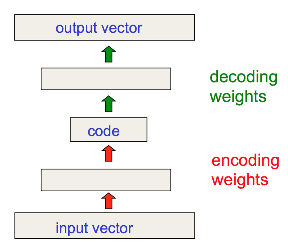
Unlike the earlier models, autoencoders are used for unsupervised learning. They are designed to learn a low-dimensional representation of a high-dimensional dataset, similar to what Principal Components Analysis (PCA) provides. An autoencoder attempts to learn an approximation function $ f(x) \approx x $ that reproduces the input data. However, it is constrained by a bottleneck layer in the middle that contains only a small number of nodes. With this limited capacity, the model is forced to form a highly efficient encoding of the data, which is essentially the low-dimensional code that it learns.

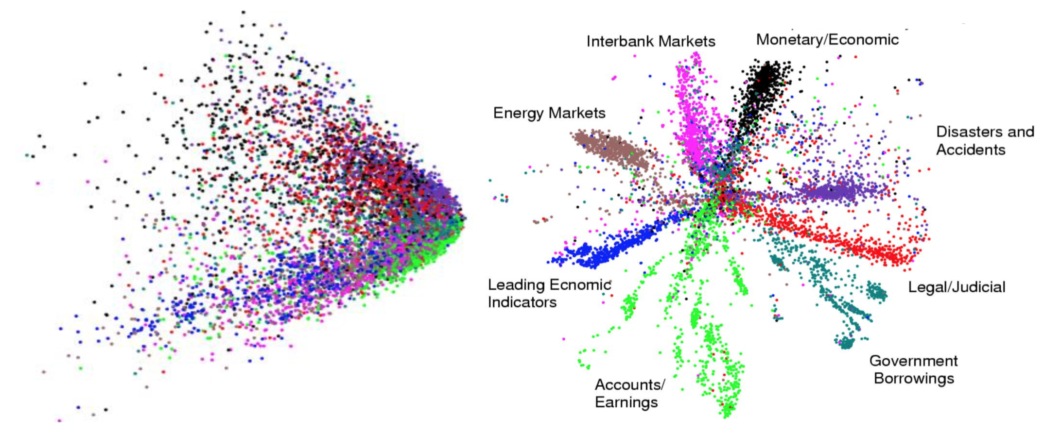
Hinton and Salakhutdinov applied autoencoders to compress documents spanning a variety of topics. As illustrated in Fig 10, when PCA and an autoencoder were both used to reduce documents to two dimensions, the autoencoder produced a substantially better result. With autoencoders, we can perform efficient data compression to accelerate information retrieval for both documents and images.

Reinforcement (Deep) Learning

Since this post opened with AlphaGo, it is worth looking more closely at why AlphaGo succeeded. Reinforcement learning (“RL”) is one of the key ingredients. RL is a subfield of machine learning that enables machines and software agents to automatically determine optimal behavior in a given context, with the objective of maximizing long-term performance as measured by a specified metric.

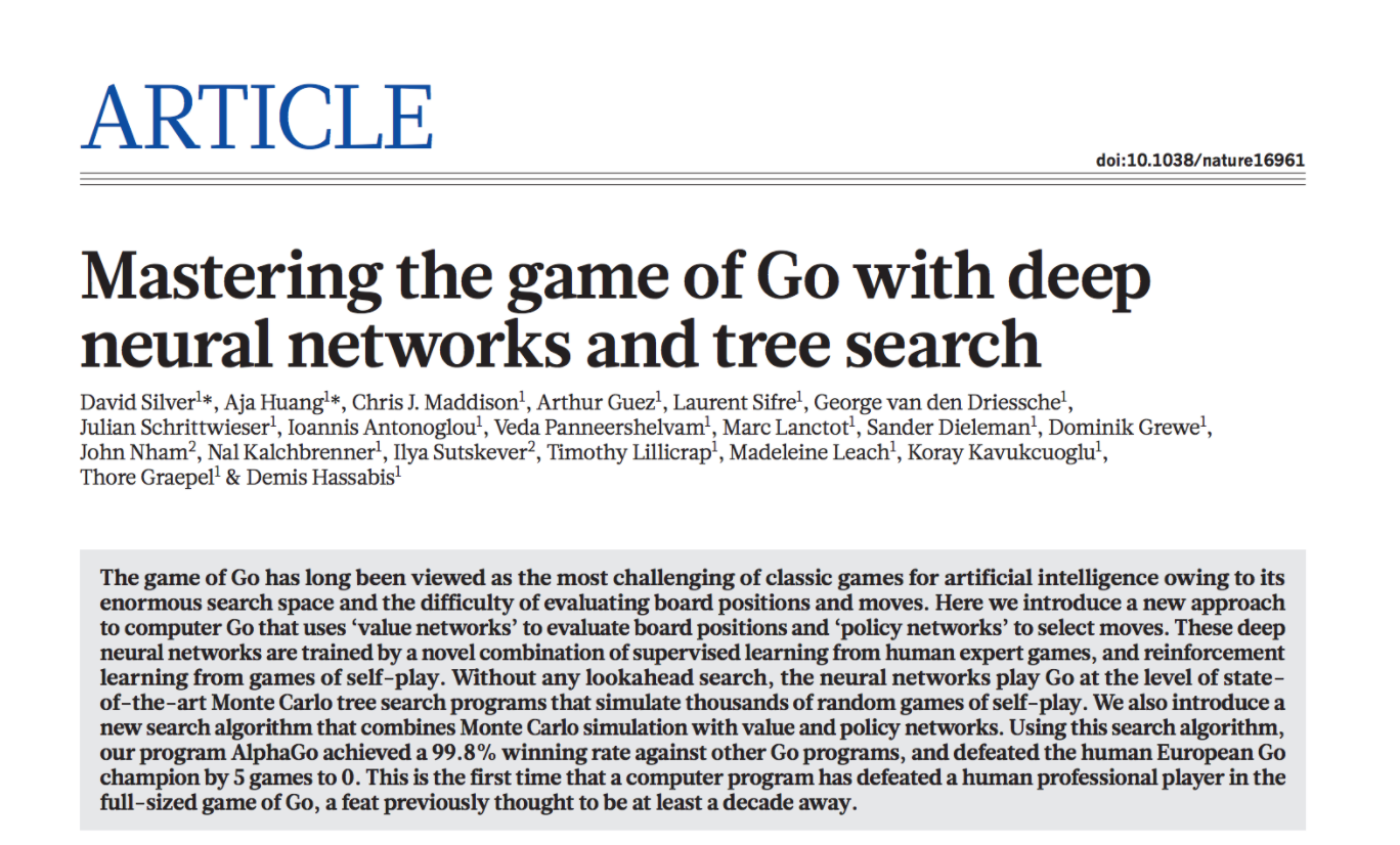
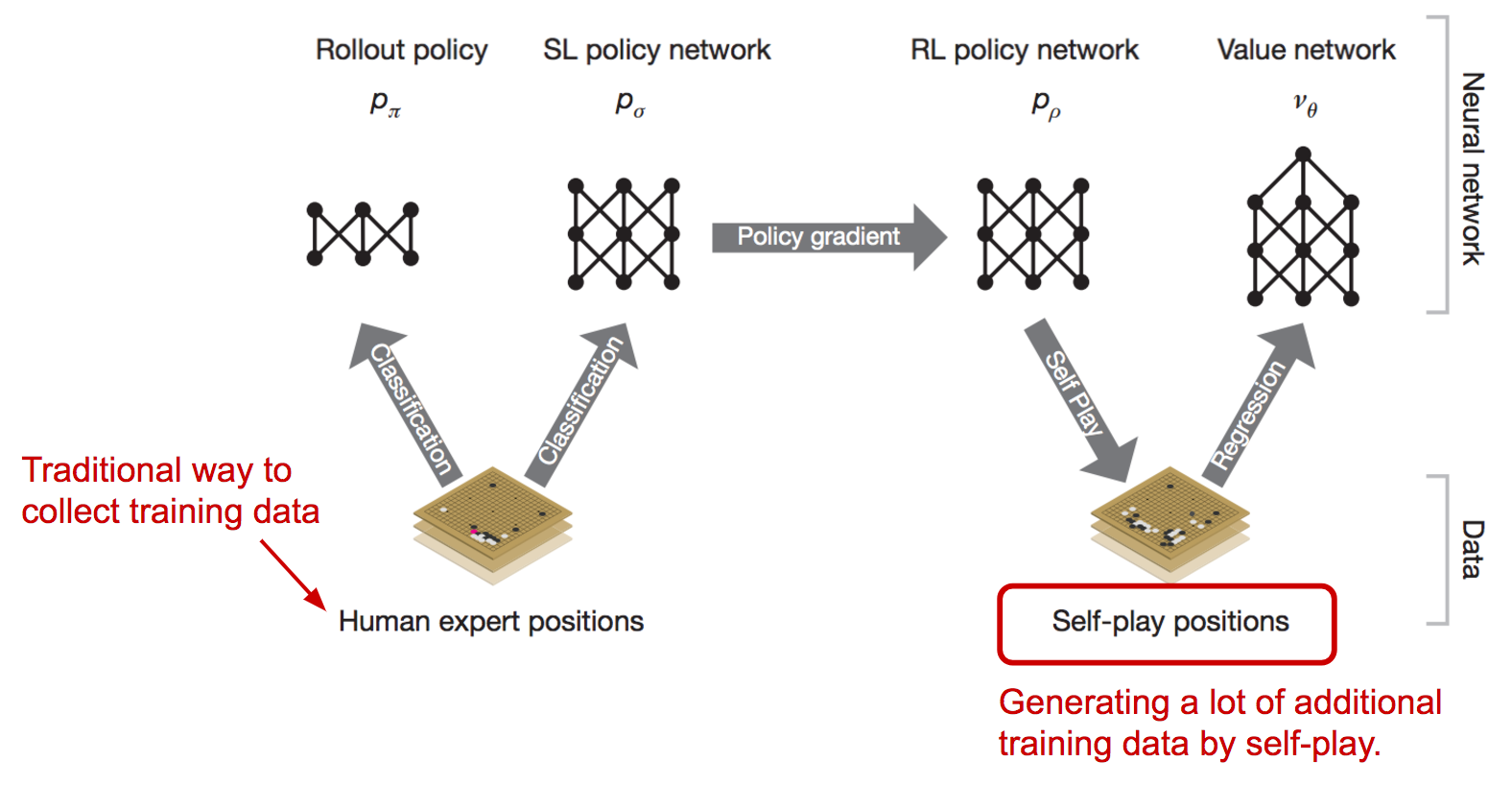
The AlphaGo system begins with supervised learning to train a fast rollout policy and a policy network, using a manually curated dataset of professional players’ games. In this stage, it learns the best strategy given the current position on the game board. It then applies reinforcement learning by running self-play games. The RL policy network improves as it wins more games against previous versions of itself. During self-play, AlphaGo becomes increasingly strong by playing against itself, without requiring additional external training data.

Generative Adversarial Network

Generative adversarial network, abbreviated “GAN,” is a type of deep generative model. A GAN can create new examples after learning from real data. It consists of two models that compete in a zero-sum game framework. The well-known deep learning researcher Yann LeCun gave it very high praise: Generative Adversarial Network is the most interesting idea in the last ten years in machine learning. (See the Quora question: “What are some recent and potentially upcoming breakthroughs in deep learning?”)

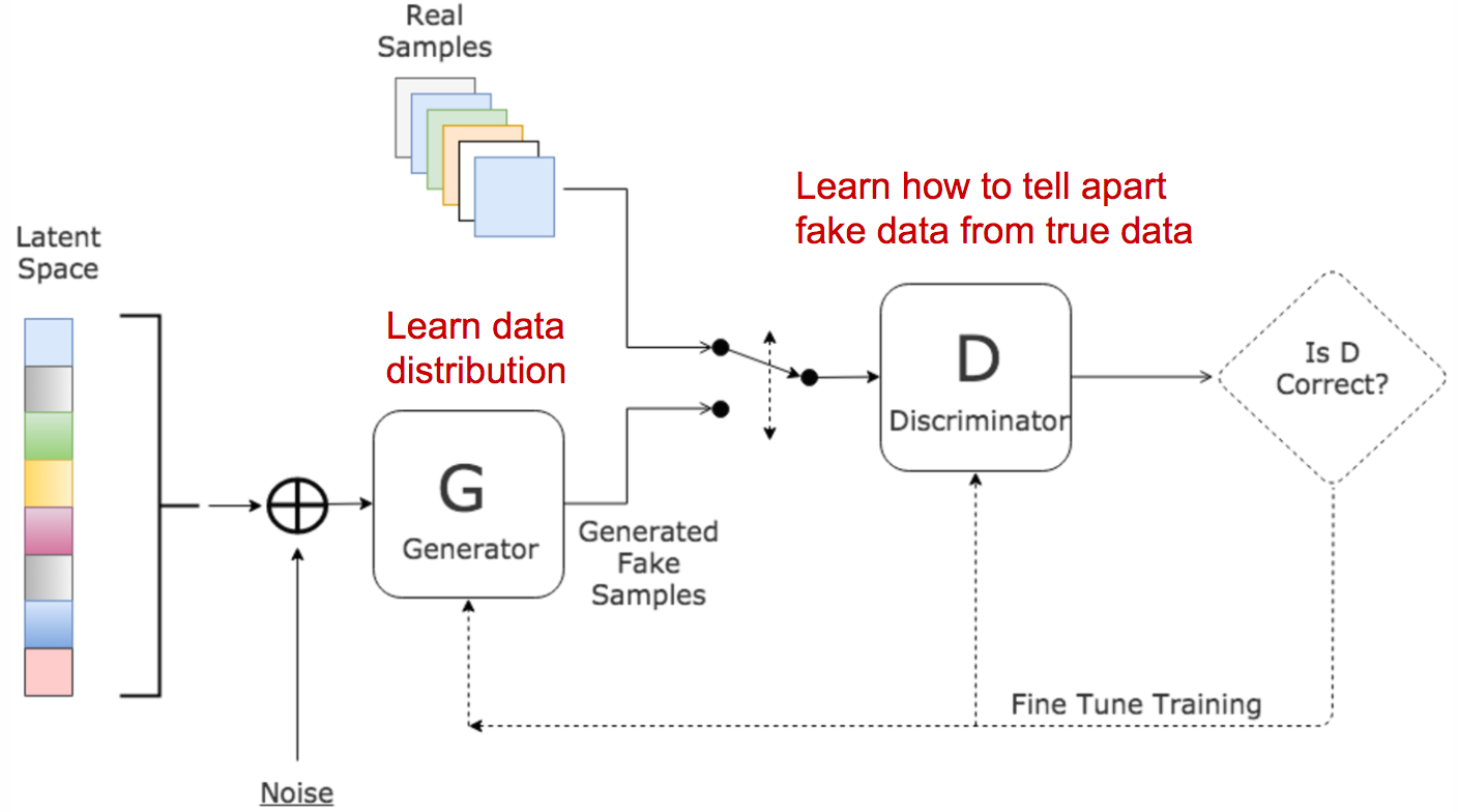
In the original GAN paper, GAN was introduced as a method for generating meaningful images after learning from real photos. It includes two separate models: the Generator and the Discriminator. The generator produces fake images and passes them to the discriminator. The discriminator acts as a judge, optimized to distinguish real photos from fake ones. The generator works to fool the discriminator, while the judge works to avoid being fooled. This zero-sum interaction encourages both models to strengthen their respective capabilities and improve performance. Ultimately, the generator is the component used to produce new images.

Toolkits and Libraries

After reviewing these models, you may be wondering how to implement them and apply them in practice. Fortunately, many open source toolkits and libraries are available for building deep learning models. Tensorflow is relatively new, yet it has quickly attracted significant popularity. Notably, TensorFlow was the most forked Github project of 2015. That occurred within a two-month period after its release in Nov 2015.

How to Learn?

If you are new to the field and willing to invest time in studying deep learning in a more systematic way, I recommend starting with the book Deep Learning by Ian Goodfellow, Yoshua Bengio, and Aaron Courville. Another strong option is Geoffrey Hinton’s Coursera course “Neural Networks for Machine Learning” (Godfather of deep learning!). The course content was prepared around 2006, so it is fairly old, but it helps build a solid foundation for understanding deep learning models and can expedite further exploration.

In addition, keep your curiosity and passion. The field advances daily. Even classical or widely adopted deep learning models may have been introduced only 1-2 years ago. Reading academic papers can help you learn topics in depth and stay current with cutting-edge findings.

Useful resources

• Google Scholar: http://scholar.google.com
• arXiv cs section: https://arxiv.org/list/cs/recent
• Unsupervised Feature Learning and Deep Learning Tutorial
• Tensorflow Tutorials
• Data Science Weekly
• KDnuggets
• Tons of blog posts and online tutorials
• Related Cousera courses
• awesome-deep-learning-papers

Blog posts mentioned

• Explained Visually: Image Kernels
• Understanding LSTM Networks
• The Unreasonable Effectiveness of Recurrent Neural Networks
• Computer, respond to this email.

Interesting blogs worthy of checking

• www.wildml.com
• colah.github.io
• karpathy.github.io
• blog.openai.com

Papers mentioned

[1] He, Kaiming, et al. “Deep residual learning for image recognition.” Proc. IEEE Conf. on computer vision and pattern recognition. 2016.

[2] Wang, Haohan, Bhiksha Raj, and Eric P. Xing. “On the Origin of Deep Learning.” arXiv preprint arXiv:1702.07800, 2017.

[3] Sutskever, Ilya, James Martens, and Geoffrey E. Hinton. “Generating text with recurrent neural networks.” Proc. of the 28th Intl. Conf. on Machine Learning (ICML). 2011.

[4] Liwicki, Marcus, et al. “A novel approach to on-line handwriting recognition based on bidirectional long short-term memory networks.” Proc. of 9th Intl. Conf. on Document Analysis and Recognition. 2007.

[5] LeCun, Yann, Yoshua Bengio, and Geoffrey Hinton. “Deep learning.” Nature 521.7553 (2015): 436-444.

[6] Hochreiter, Sepp, and Jurgen Schmidhuber. “Long short-term memory.” Neural computation 9.8 (1997): 1735-1780.

[7] Cho, Kyunghyun. et al. “Learning phrase representations using RNN encoder-decoder for statistical machine translation.” Proc. Conference on Empirical Methods in Natural Language Processing 1724–1734 (2014).

[8] Hinton, Geoffrey E., and Ruslan R. Salakhutdinov. “Reducing the dimensionality of data with neural networks.” science 313.5786 (2006): 504-507.

[9] Silver, David, et al. “Mastering the game of Go with deep neural networks and tree search.” Nature 529.7587 (2016): 484-489.

[10] Goodfellow, Ian, et al. “Generative adversarial nets.” NIPS, 2014.