Anatomize Deep Learning with Information Theory
Professor Naftali Tishby passed away in 2021. I hope this post will introduce his compelling idea of the information bottleneck to a wider audience. Recently, I watched Prof. Naftali Tishby’s talk, “Information Theory in Deep Learning,” and found it highly engaging. In the talk, he explained how information theory can be used to examine the growth and transformation of deep neural networks during training. Using the Information Bottleneck (IB) method, he proposed a new learning bound for deep neural networks (DNN), since traditional learning theory breaks down in the presence of an exponentially large number of parameters. He also highlighted a sharp observation about DNN training: it proceeds in two distinct phases. First, the network is trained to fully represent the input data and to minimize the generalization error; next, it learns to discard irrelevant details by compressing the input representation.
· 9 min read · Curated and presented by Arthur Sedek
Professor Naftali Tishby passed away in 2021. Hope the post can introduce his cool idea of information bottleneck to more people.
I recently watched “Information Theory in Deep Learning” by Professor Naftali Tishby and found it compelling. He describes how information theory can be applied to study how deep neural networks evolve while training. Using the Information Bottleneck (IB) framework, he proposes a new learning bound for deep neural networks (DNNs), motivated by the fact that traditional learning theory breaks down in the presence of an exponentially large number of parameters. He also highlights an important empirical pattern: DNN training appears to proceed in two distinct phases. First, the network learns to represent the input data and reduce generalization error; afterward, it begins to discard irrelevant details by compressing its input representation.
Most of the content in this post is drawn from Professor Tishby’s talk and the related papers.
Basic Concepts
A Markov process is a “memoryless” stochastic process (also referred to as the “Markov Property”). A Markov chain is a Markov process with multiple discrete states. In other words, the conditional probability of future states depends only on the current state and is independent of all past states.
Kullback–Leibler (KL) Divergence
KL divergence quantifies how one probability distribution $p$ differs from a second, reference probability distribution $q$. It is not symmetric.
$D_{KL}$ attains its minimum value of zero when $p(x)$ == $q(x)$ everywhere.
Mutual information measures the statistical dependence between two variables. It expresses the “amount of information” gained about one random variable from observing the other. Mutual information is symmetric.
Data Processing Inequality (DPI)
For any Markov chain $X \to Y \to Z$, we have $I(X; Y) \geq I(X; Z)$.
A deep neural network can be interpreted as a Markov chain. Therefore, as we move through the layers of a DNN, the mutual information between a given layer and the input can only decrease.
Given two invertible functions $\phi$ and $\psi$, mutual information remains unchanged: $I(X; Y) = I(\phi(X); \psi(Y))$.
For instance, shuffling the weights within a DNN layer does not change the mutual information between that layer and another layer.
Deep Neural Networks as Markov Chains
The training set contains sampled observations from the joint distribution of $X$ and $Y$. The input variable $X$ and the hidden-layer weights are high-dimensional random variables. In classification settings, the ground-truth target $Y$ and the predicted output $\hat{Y}$ are lower-dimensional random variables.
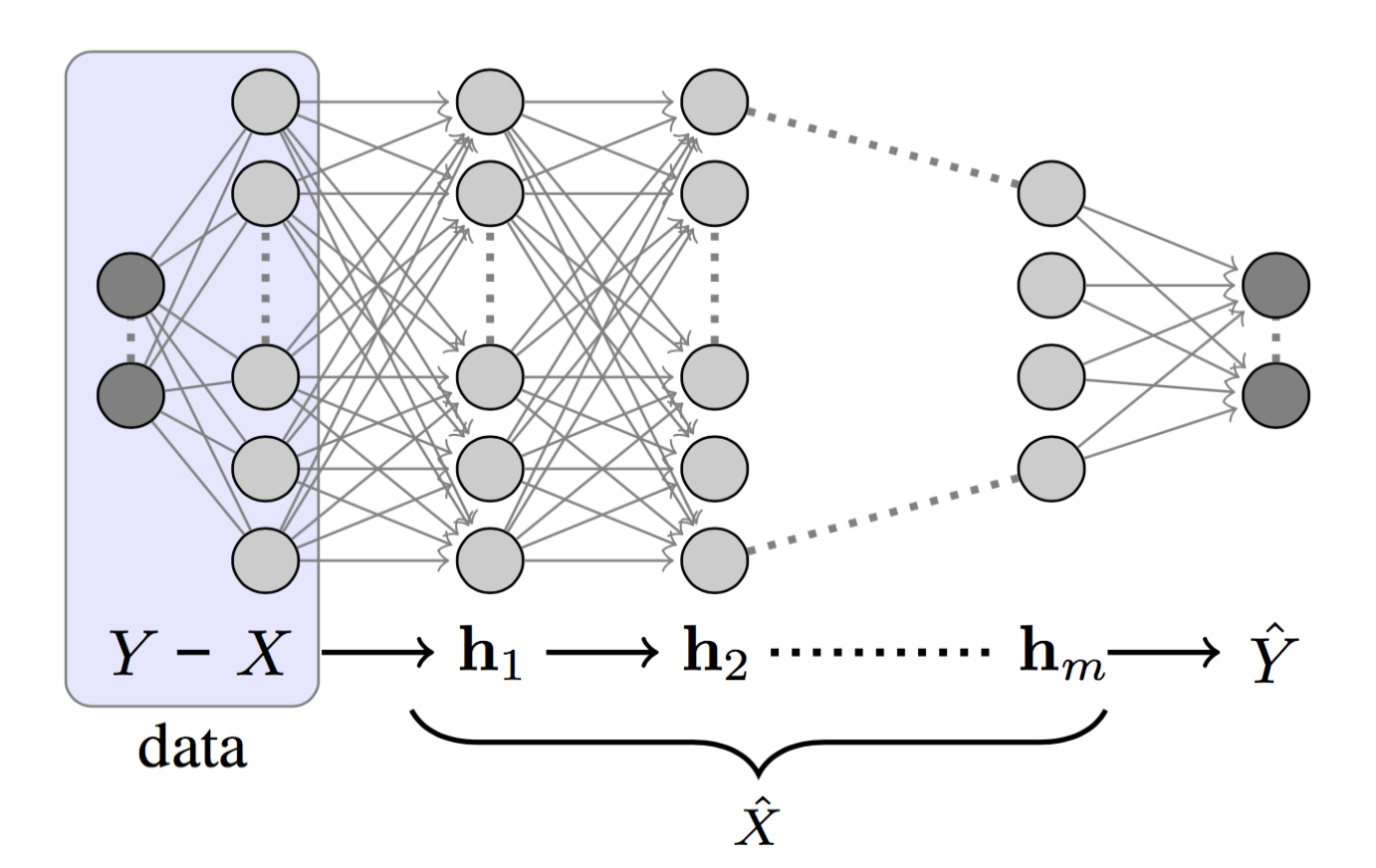
If we denote the hidden layers as $h_1, h_2, \dots, h_m$, as in Fig. 1, then each layer can be treated as a state in a Markov chain: $ h_i \to h_{i+1}$. By DPI, it follows that:
A DNN is built to learn an effective description of $X$ in order to predict $Y$ and, ultimately, to compress $X$ so that it retains only the information relevant to $Y$. Tishby refers to this sequence of transformations as “successive refinement of relevant information”.
Information Plane Theorem
A DNN forms successive internal representations of $X$ across its hidden layers $\{T_i\}$. The information plane theorem characterizes each layer using encoder and decoder information. The encoder represents the input $X$, while the decoder maps the current layer’s representation to the target output $Y$.
More specifically, in an information plane plot:
- X-axis: The sample complexity of $T_i$ is determined by the encoder mutual information $I(X; T_i)$. Sample complexity describes how many samples are required to reach a given accuracy and generalization level.
- Y-axis: The accuracy (generalization error) is determined by the decoder mutual information $I(T_i; Y)$.
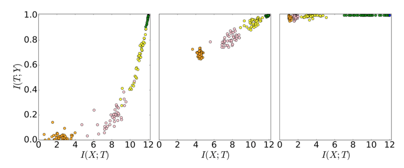
Each dot marks the encoder and decoder mutual information of a single hidden layer from one network simulation (with no regularization applied, no weight decay, no dropout, etc.). As expected, the points move upward because the model’s information about the true labels increases (and accuracy improves). Early in training, hidden layers learn substantial information about the input $X$, but later they begin to compress, discarding some input information. Tishby argues that “the most important part of learning is actually forgetting”. See this nice video for a visualization of how the layers’ mutual information evolves over epochs.
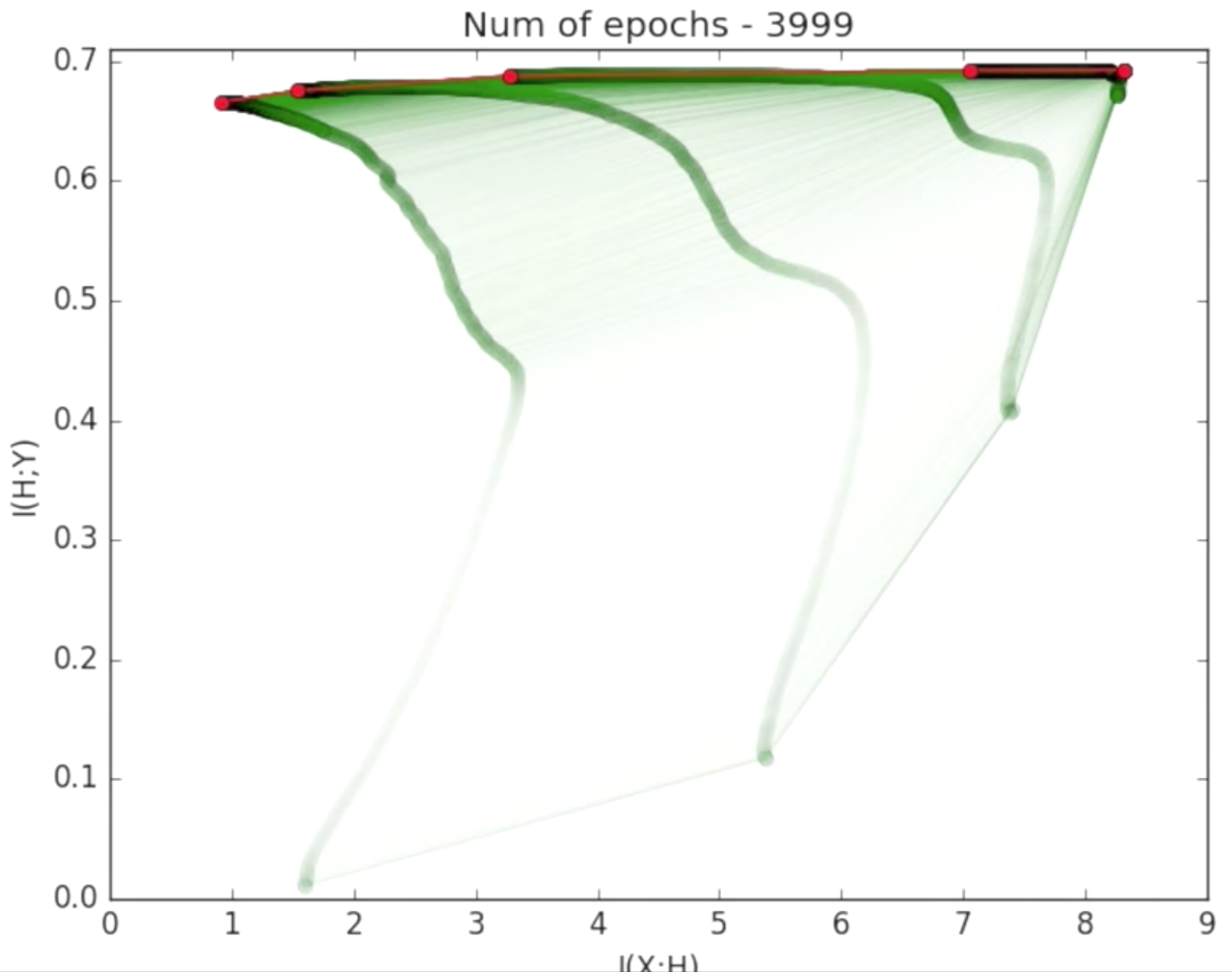
Two Optimization Phases
Two optimization phases also become apparent when tracking the normalized mean and standard deviation of each layer’s weights over time.
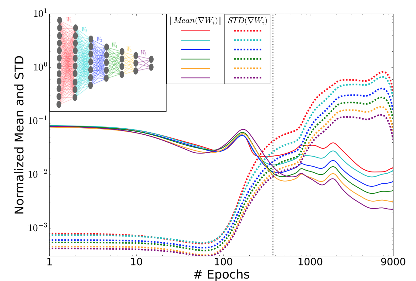
During early epochs, the mean values are three orders of magnitude larger than the standard deviations. After enough epochs, the error saturates and the standard deviations subsequently become much noisier. The farther a layer is from the output, the noisier it becomes, because noise can be amplified and accumulated through backpropagation (rather than being caused by the layer’s width).
Learning Theory
“Old” Generalization Bounds
Classic learning theory defines the generalization bound as:
- $\epsilon$: The gap between training error and generalization error. Generalization error measures how accurately an algorithm predicts on previously unseen data.
- $H_\epsilon$: A $\epsilon$-cover of the hypothesis class. Typically, we assume size $\vert H_\epsilon \vert \sim (1/\epsilon)^d$.
- $\delta$: Confidence.
- $m$: The number of training samples.
- $d$: The VC dimension of the hypothesis.
This formulation states that the difference between training error and generalization error is bounded by a function of the hypothesis-space size and the dataset size. As the hypothesis space grows, the bound becomes looser, implying a larger generalization gap. For additional background on generalization bounds, see this ML theory tutorial, part1 and part2.
However, this approach does not align well with deep learning. Larger networks contain more parameters, and under these bounds, larger models (larger $d$) would yield worse guarantees. This conflicts with the common intuition that larger networks often perform better because of their greater expressivity.
“New” Input compression bound
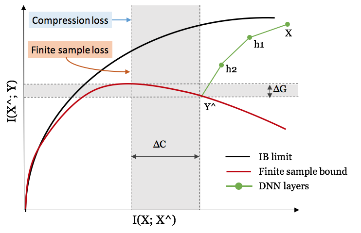
To address this counterintuitive outcome, Tishby et al. propose a new input-compression bound for DNNs.
Let $T_\epsilon$ be an $\epsilon$-partition of the input variable $X$. This partition compresses the input by grouping it into small cells according to label homogeneity. Collectively, the cells cover the full input space. When prediction outputs are binary, the hypothesis cardinality $\vert H_\epsilon \vert$ can be replaced by $2^{\vert T_\epsilon \vert}$.
When $X$ is large, the size of $X$ is approximately $2^{H(X)}$. Each cell in the $\epsilon$-partition has size $2^{H(X \vert T_\epsilon)}$. Hence, we obtain $\vert T_\epsilon \vert \sim \frac{2^{H(X)}}{2^{H(X \vert T_\epsilon)}} = 2^{I(T_\epsilon; X)}$. The resulting input-compression bound is:
Network Size and Training Data Size
The Benefit of More Hidden Layers
Adding layers provides computational benefits and can accelerate training toward good generalization.
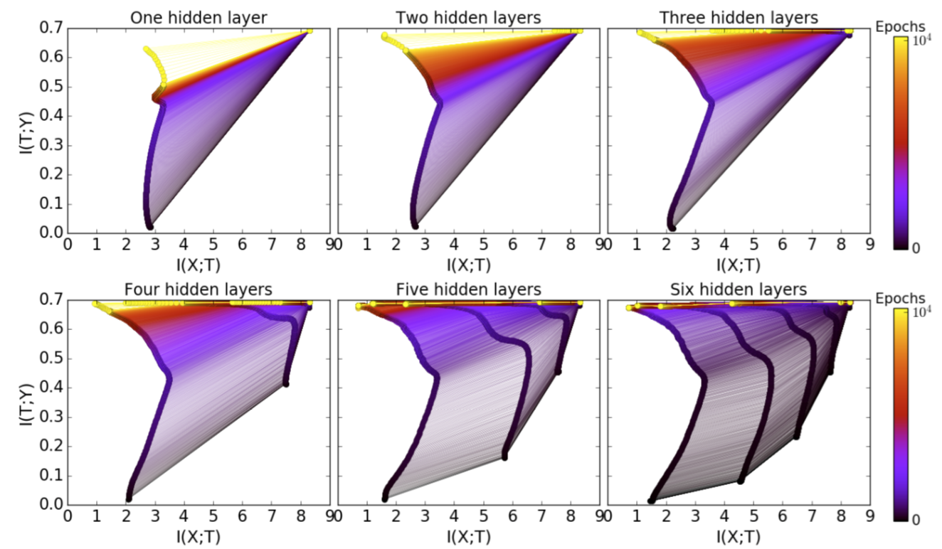
Compression through stochastic relaxation: Based on the diffusion equation, the relaxation time of layer $k$ is proportional to the exponential of the layer’s compression amount $\Delta S_k$: $\Delta t_k \sim \exp(\Delta S_k)$. The layer compression can be computed as $\Delta S_k = I(X; T_k) - I(X; T_{k-1})$. Because $\exp(\sum_k \Delta S_k) \geq \sum_k \exp(\Delta S_k)$, we would expect training epochs to decrease exponentially as the number of hidden layers increases (larger $k$).
The Benefit of More Training Samples
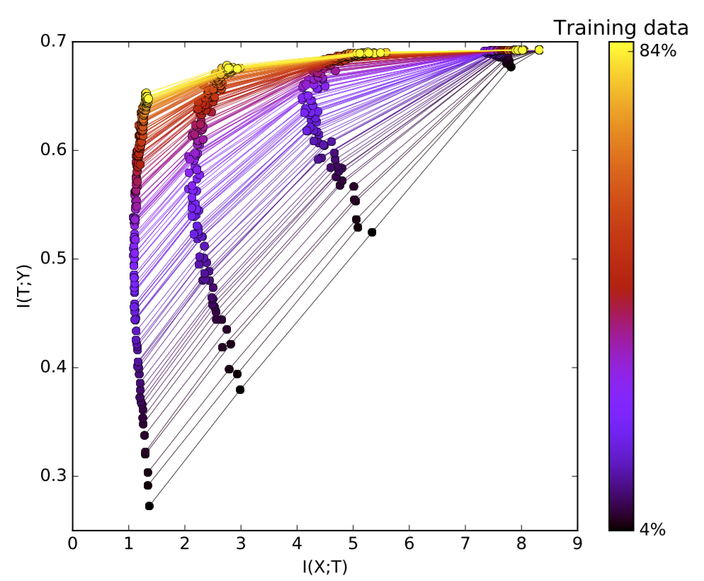
Fitting more training data requires the hidden layers to capture more information. As the training dataset grows, the decoder mutual information (which, recall, is directly tied to generalization error) $I(T; Y)$ is pushed upward and approaches the theoretical information bottleneck bound. Tishby emphasizes that mutual information, rather than layer size or VC dimension, determines generalization, in contrast to standard theories.
Cited as:
@article{weng2017infotheory,
  title   = "Anatomize Deep Learning with Information Theory",
  author  = "Weng, Lilian",
  journal = "lilianweng.github.io",
  year    = "2017",
  url     = "https://lilianweng.github.io/posts/2017-09-28-information-bottleneck/"
}
References
[1] Naftali Tishby. Information Theory of Deep Learning
[2] Machine Learning Theory - Part 1: Introduction
[3] Machine Learning Theory - Part 2: Generalization Bounds
[4] New Theory Cracks Open the Black Box of Deep Learning by Quanta Magazine.
[5] Naftali Tishby and Noga Zaslavsky. “Deep learning and the information bottleneck principle.” IEEE Information Theory Workshop (ITW), 2015.
[6] Ravid Shwartz-Ziv and Naftali Tishby. “Opening the Black Box of Deep Neural Networks via Information.” arXiv preprint arXiv:1703.00810, 2017.