Learning Word Embedding
Human language is expressed as free text. To enable a machine learning model to interpret and process natural language, we must convert free-text words into numeric representations. One of the simplest approaches is one-hot encoding, where each unique word corresponds to a single dimension in the resulting vector, and a binary value indicates whether the word is present (1) or absent (0).
· 18 min read · Curated and presented by Arthur Sedek
Human vocabulary is expressed as free text. To enable a machine learning model to interpret and process natural language, we must convert free-text words into numeric values. One of the simplest approaches is one-hot encoding, where each distinct word corresponds to one dimension in the resulting vector, and a binary value indicates whether the word is present (1) or absent (0).
However, one-hot encoding becomes computationally impractical for a full vocabulary because it requires hundreds of thousands of dimensions. Word embeddings instead represent words and phrases as vectors of (non-binary) numeric values with far fewer dimensions, producing a denser representation. A natural expectation for high-quality embeddings is that they approximate similarity between words (for example, “cat” and “kitten” should be close in the reduced vector space) and reveal hidden semantic relationships (for example, the relationship between “cat” and “kitten” parallels the relationship between “dog” and “puppy”). Context is particularly valuable for learning meaning and relationships, because similar words often appear in similar contexts.
There are two primary approaches to learning word embeddings, and both rely on contextual information.
- Count-based: This approach is unsupervised and uses matrix factorization on a global word co-occurrence matrix. Because raw co-occurrence counts tend to perform poorly, additional techniques are typically applied to improve them.
- Context-based: This approach is supervised. Given a local context, we design a model to predict target words; during training, the model simultaneously learns an efficient word embedding representation.
Count-Based Vector Space Model
Count-based vector space models depend heavily on word frequency and a co-occurrence matrix, based on the assumption that words appearing in the same contexts share similar or related semantic meanings. These models compress count-based statistics, such as co-occurrence patterns among neighboring words, into small, dense word vectors. PCA, topic models, and neural probabilistic language models are all representative examples in this category.
In contrast to count-based approaches, context-based methods construct predictive models that explicitly aim to predict a word from its neighbors. The dense word vectors are included as model parameters, and an effective vector representation for each word is learned as part of training.
Context-Based: Skip-Gram Model
Assume a fixed-size sliding window moves across a sentence: the center word is the “target,” and the words to its left and right within the window are the context words. The skip-gram model (Mikolov et al., 2013) is trained to predict the probability that a word appears as a context word given a target.
The example below shows several target-context word pairs used as training samples, generated by sliding a 5-word window over the sentence.
“The man who passes the sentence should swing the sword.” – Ned Stark
| Sliding window (size = 5) | Target word | Context |
|---|---|---|
| [The man who] | the | man, who |
| [The man who passes] | man | the, who, passes |
| [The man who passes the] | who | the, man, passes, the |
| [man who passes the sentence] | passes | man, who, the, sentence |
| … | … | … |
| [sentence should swing the sword] | swing | sentence, should, the, sword |
| [should swing the sword] | the | should, swing, sword |
| [swing the sword] | sword | swing, the |
| {:.info} |
Each context-target pair is treated as a separate observation in the dataset. For instance, in the example above, the target word “swing” yields four training samples: (“swing”, “sentence”), (“swing”, “should”), (“swing”, “the”), and (“swing”, “sword”).
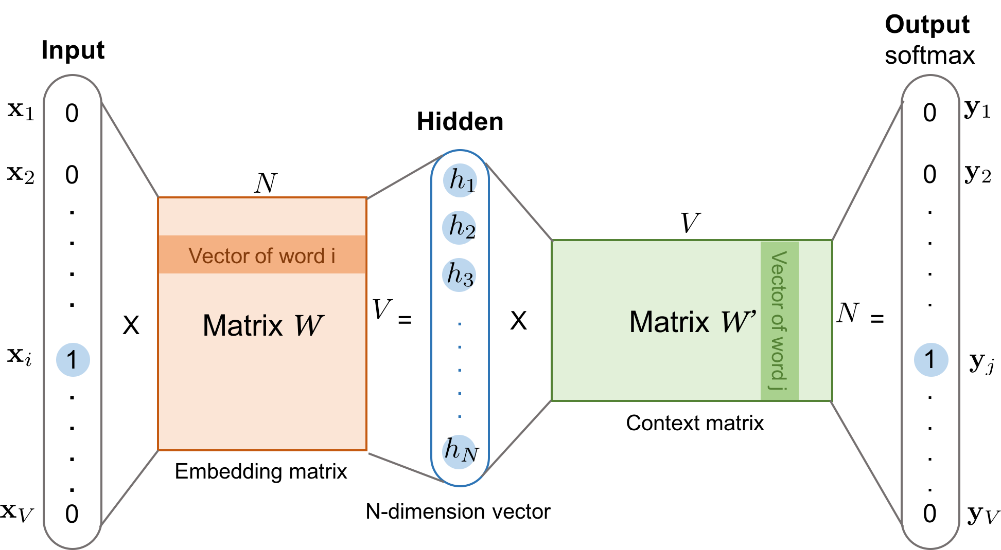
Given the vocabulary size $V$, we aim to learn word embedding vectors of size $N$. The model predicts one context word (output) from one target word (input) at a time.
As shown in Fig. 1:
- The input word $w_i$ and the output word $w_j$ are both one-hot encoded as binary vectors $\mathbf{x}$ and $\mathbf{y}$, each of size $V$.
- First, multiplying the binary vector $\mathbf{x}$ by the word embedding matrix $W$ (of size $V \times N$) yields the embedding vector for the input word $w_i$, namely the i-th row of the matrix $W$.
- This newly obtained embedding vector, with dimension $N$, constitutes the hidden layer.
- Multiplying the hidden layer by the word context matrix $W’$ (of size $N \times V$) produces the output one-hot encoded vector $\mathbf{y}$.
- The output context matrix $W’$ represents word meaning in the role of context, and it differs from the embedding matrix $W$. NOTE: Despite the naming, $W’$ is independent of $W$, it is not a transpose, inverse, or anything similar.
Context-Based: Continuous Bag-of-Words (CBOW)
Continuous Bag-of-Words (CBOW) is another closely related model for learning word vectors. It predicts the target word (for example, “swing”) from the source context words (for example, “sentence should the sword”).
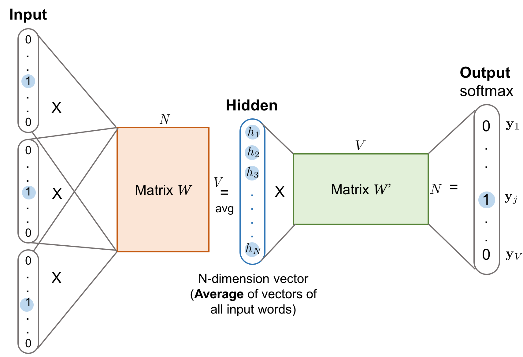
Because there are multiple context words, we average their corresponding word vectors, which are constructed by multiplying the input vector by the matrix $W$. Since averaging smooths out substantial distributional information, some believe CBOW performs better on smaller datasets.
Loss Functions
Both skip-gram and CBOW are trained by minimizing a carefully designed loss (objective) function. Multiple loss functions can be used to train these language models. In the discussion below, we use skip-gram as the running example for how the loss is computed.
Full Softmax
The skip-gram model defines each word’s embedding vector through the matrix $W$ and each word’s context vector through the output matrix $W’$. Given an input word $w_I$, we denote the corresponding row of $W$ as vector $v_{w_I}$ (the embedding vector) and the corresponding column of $W’$ as $v’_{w_I}$ (the context vector). The output layer applies softmax to compute the probability of predicting output word $w_O$ given $w_I$; therefore:
This is accurate as presented in However, when $V$ is extremely large, computing the denominator by iterating over all words for every training sample becomes computationally infeasible. The need for more efficient conditional probability estimation motivates methods such as hierarchical softmax.
Hierarchical Softmax
Morin and Bengio (2005) proposed hierarchical softmax to accelerate the summation using a binary tree. Hierarchical softmax encodes the language model’s output softmax layer as a tree: each leaf corresponds to a word, and each internal node represents the relative probabilities of its child nodes.
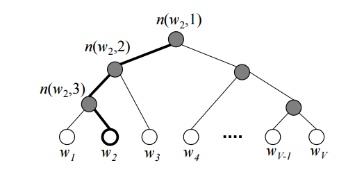
Each word $w_i$ has a unique path from the root to its corresponding leaf. The probability of selecting that word equals the probability of traversing the associated path from the root through the branches. Given the embedding vector $v_n$ for internal node $n$, the word probability can be computed as the product of the probabilities of taking the left or right branch at each internal node along the path.
As in Fig. 3, the probability at a node is ($\sigma$ is the sigmoid function):
The resulting probability of producing a context word $w_O$ given an input word $w_I$ is:
where $L(w_O)$ is the depth of the path to word $w_O$, and $\mathbb{I}_{\text{turn}}$ is a special indicator function that returns 1 if $n(w_O, k+1)$ is the left child of $n(w_O, k)$, and otherwise returns -1. The embeddings of internal nodes are learned during training. This tree structure substantially reduces the complexity of estimating the denominator from O(V) (vocabulary size) to O(log V) (tree depth) during training. However, at prediction time, we still to compute the probability of every word and select the best, because the target leaf is not known in advance.
The choice of tree structure is important for model quality. Useful guiding principles include grouping words by frequency (as in a Huffman tree) for a simple speedup, and grouping semantically similar words into the same or nearby branches (for example, using predefined word clusters or WordNet).
Morin and Bengio use the synsets in WordNet as clusters for the tree. Mnih and Hinton learn the tree structure with a clustering algorithm that recursively partitions the words in two clusters.Cross Entropy
Another option avoids the softmax framework entirely. Instead, the loss measures cross entropy between the predicted probabilities $p$ and the true binary labels $\mathbf{y}$.
First, recall that the cross entropy between two distributions $p$ and $q$ is measured as $ H(p, q) = -\sum_x p(x) \log q(x) $. In our setting, the true label $y_i$ equals 1 only when $w_i$ is the output word; otherwise $y_j$ equals 0. The model’s loss $\mathcal{L}_\theta$, under parameter configuration $\theta$, minimizes the cross entropy between predictions and ground truth, since lower cross entropy implies greater similarity between the two distributions.
Recall that:
Therefore:
To begin training with back-propagation and SGD, we need the gradient of the loss. For simplicity, let’s denote $z_{IO} = {v’_{w_O}}^{\top}{v_{w_I}}$.
where $Q(\tilde{w})$ is the noise-sample distribution.
From the expression above, the correct output word receives positive reinforcement from the first term (the larger $\nabla_\theta z_{IO}$, the better the loss), while other words contribute negatively via the second term.
Estimating $\mathbb{E}_{w_i \sim Q(\tilde{w})} \nabla_\theta {v’_{w_i}}^{\top}{v_{w_I}}$ using a set of sampled noise words, rather than iterating over the entire vocabulary, is the core idea behind cross-entropy-based sampling approaches.
Noise Contrastive Estimation (NCE)
Noise Contrastive Estimation (NCE) trains a logistic regression classifier to distinguish the true target word from noise samples (Gutmann and Hyvärinen, 2010).
Given an input word $w_I$, the correct output word is $w$. At the same time, we sample $N$ additional words from the noise distribution $Q$, denoted as $\tilde{w}_1, \tilde{w}_2, \dots, \tilde{w}_N \sim Q$. Let the binary classifier’s decision be $d$, and $d$ can only take a binary value.
When $N$ is sufficiently large, by the Law of large numbers:
To compute probability $p(d=1 \vert w, w_I)$, we begin with the joint probability $p(d, w \vert w_I)$. Among $w, \tilde{w}_1, \tilde{w}_2, \dots, \tilde{w}_N$, there is a 1 out of (N+1) chance to select the true word $w$, which is sampled from conditional probability $p(w \vert w_I)$. Meanwhile, there are N out of (N+1) chances to select a noise word, each sampled from $q(\tilde{w}) \sim Q$. Thus:
From this, we can derive $p(d=1 \vert w, w_I)$ and $p(d=0 \vert w, w_I)$:
The resulting loss function for NCE’s binary classifier is:
However, $p(w \vert w_I)$ still requires summing over the entire vocabulary in the denominator. Let’s denote that denominator as the partition function for the input word, $Z(w_I)$. A common assumption is $Z(w) \approx 1$, because we expect the softmax output layer to be normalized (Minh and Teh, 2012). Under this assumption, the loss simplifies to:
The noise distribution $Q$ is a tunable parameter, and it is typically designed so that:
- it is intuitively similar to the true data distribution, and
- it is straightforward to sample from.
For example, the NCE loss sampling implementation in tensorflow (log_uniform_candidate_sampler) assumes a log-uniform noise distribution, also called Zipfian’s law. The log-probability of a word is assumed to be inversely proportional to its rank, with higher-frequency words assigned lower ranks. In this setting, $q(\tilde{w}) = \frac{1}{ \log V}(\log (r_{\tilde{w}} + 1) - \log r_{\tilde{w}})$, where $r_{\tilde{w}} \in [1, V]$ is the frequency rank of the word in descending order.
Negative Sampling (NEG)
Negative Sampling (NEG), proposed by Mikolov et al. (2013), is a simplified variant of NCE loss. It is widely known for its use in Google’s word2vec project. Unlike NCE loss, which aims to approximately maximize the log probability of the softmax output, negative sampling applies further simplifications because it targets high-quality word embeddings rather than accurate modeling of the full word distribution in natural language.
NEG approximates the binary classifier output using sigmoid functions as follows:
The final NCE loss function looks like:
Other Tips for Learning Word Embedding
Mikolov et al. (2013) suggested several practical techniques that can improve word embedding learning outcomes.
-
Soft sliding window. When forming word pairs within a sliding window, it can be useful to assign less weight to words that are farther away. One heuristic is: given a maximum window size parameter $s_{\text{max}}$, the actual window size is randomly sampled between 1 and $s_{\text{max}}$ for each training example. As a result, each context word is observed with probability 1/(its distance to the target word), while adjacent words are always observed.
-
Subsampling frequent words. Very frequent words can be too generic to provide distinctive contextual signals (for example, stopwords). Conversely, rare words are more likely to carry specific information. To balance frequent and rare terms, Mikolov et al. proposed discarding words $w$ with probability $1-\sqrt{t/f(w)}$ during sampling. Here $f(w)$ is the word frequency, and $t$ is an adjustable threshold.
-
Learning phrases first. A phrase often functions as a single conceptual unit rather than a simple composition of individual words. For example, even if we know the meanings of “new” and “york,” we cannot reliably infer that “New York” is a city name. Learning such phrases first and treating them as word units before training the embedding model can improve output quality. A simple data-driven method uses unigram and bigram counts: $s_{\text{phrase}} = \frac{C(w_i w_j) - \delta}{ C(w_i)C(w_j)}$, where $C(.)$ is the raw count of a unigram $w_i$ or bigram $w_i w_j$, and $\delta$ is a discounting threshold intended to prevent extremely infrequent words and phrases from being selected. Higher scores imply a greater likelihood that the token pair forms a phrase. To construct phrases longer than two words, we can scan the vocabulary multiple times while gradually lowering the score cutoff.
GloVe: Global Vectors
The Global Vectors (GloVe) model proposed by Pennington et al. (2014) is intended to combine count-based matrix factorization with the context-based skip-gram model.
Counts and co-occurrences are well known to encode word meaning. To distinguish from $p(w_O \vert w_I)$ in the context of a word embedding word, we define the co-occurrence probability as:
$C(w_i, w_k)$ counts the co-occurrence between words $w_i$ and $w_k$.
Consider two words, $w_i$=“ice” and $w_j$=“steam”. A third word $\tilde{w}_k$=“solid” is related to “ice” but not “steam”, so we expect $p_{\text{co}}(\tilde{w}_k \vert w_i)$ to be much larger than $p_{\text{co}}(\tilde{w}_k \vert w_j)$, and therefore $\frac{p_{\text{co}}(\tilde{w}_k \vert w_i)}{p_{\text{co}}(\tilde{w}_k \vert w_j)}$ should be very large. If the third word $\tilde{w}_k$ = “water” is related to both, or $\tilde{w}_k$ = “fashion” is related to neither, then $\frac{p_{\text{co}}(\tilde{w}_k \vert w_i)}{p_{\text{co}}(\tilde{w}_k \vert w_j)}$ is expected to be close to one.
The key intuition is that meanings are better captured by ratios of co-occurrence probabilities than by the probabilities themselves. The global vector formulation models the relationship between two words with respect to a third context word as:
Further, because the objective is to learn meaningful word vectors, $F$ is constructed as a function of the linear difference between two words $w_i - w_j$:
Taking into account that $F$ is symmetric between target words and context words, the final solution models $F$ as an exponential function. For additional details of the equations, please refer to the original paper (Pennington et al., 2014).
Finally:
Because the second term $-\log C(w_i)$ does not depend on $k$, we can introduce a bias term $b_i$ for $w_i$ to capture $-\log C(w_i)$. To maintain symmetry, we also introduce bias $\tilde{b}_k$ for $\tilde{w}_k$.
The GloVe loss function is designed to preserve the relationship above by minimizing the sum of squared errors:
The weighting scheme $f(c)$ is a function of the co-occurrence between $w_i$ and $w_j$, and it is a configurable model component. It should approach zero as $c \to 0$; it should be non-decreasing because higher co-occurrence should exert greater influence; and it should saturate when $c$ becomes extremely large. The paper proposes the following weighting function:
Examples: word2vec on “Game of Thrones”
After reviewing the theory above, let’s run a small experiment to derive word embeddings from “the Games of Thrones corpus”. Using gensim, the workflow is quite straightforward.
Step 1: Extract words
import sys
from nltk.corpus import stopwords
from nltk.tokenize import sent_tokenize

STOP_WORDS = set(stopwords.words('english'))

def get_words(txt):
    return filter(
        lambda x: x not in STOP_WORDS,
        re.findall(r'\b(\w+)\b', txt)
    )

def parse_sentence_words(input_file_names):
   """Returns a list of a list of words. Each sublist is a sentence."""
    sentence_words = []
    for file_name in input_file_names:
        for line in open(file_name):
            line = line.strip().lower()
            line = line.decode('unicode_escape').encode('ascii','ignore')
            sent_words = map(get_words, sent_tokenize(line))
            sent_words = filter(lambda sw: len(sw) > 1, sent_words)
            if len(sent_words) > 1:
                sentence_words += sent_words
    return sentence_words

# You would see five .txt files after unzip 'a_song_of_ice_and_fire.zip'
input_file_names = ["001ssb.txt", "002ssb.txt", "003ssb.txt",
                    "004ssb.txt", "005ssb.txt"]
GOT_SENTENCE_WORDS= parse_sentence_words(input_file_names)
Step 2: Train a word2vec model
from gensim.models import Word2Vec

# size: the dimensionality of the embedding vectors.
# window: the maximum distance between the current and predicted word within a sentence.
model = Word2Vec(GOT_SENTENCE_WORDS, size=128, window=3, min_count=5, workers=4)
model.wv.save_word2vec_format("got_word2vec.txt", binary=False)
Step 3: Validate the results
Within the GoT word-embedding space, the most similar terms to “king” and “queen” are as follows:
model.most_similar('king', topn=10)(word, similarity with ‘king’) |
model.most_similar('queen', topn=10)(word, similarity with ‘queen’) |
|---|---|
| (‘kings’, 0.897245) | (‘cersei’, 0.942618) |
| (‘baratheon’, 0.809675) | (‘joffrey’, 0.933756) |
| (‘son’, 0.763614) | (‘margaery’, 0.931099) |
| (‘robert’, 0.708522) | (‘sister’, 0.928902) |
| (’lords’, 0.698684) | (‘prince’, 0.927364) |
| (‘joffrey’, 0.696455) | (‘uncle’, 0.922507) |
| (‘prince’, 0.695699) | (‘varys’, 0.918421) |
| (‘brother’, 0.685239) | (’ned’, 0.917492) |
| (‘aerys’, 0.684527) | (‘melisandre’, 0.915403) |
| (‘stannis’, 0.682932) | (‘robb’, 0.915272) |
Cited as:
@article{weng2017wordembedding,
  title   = "Learning word embedding",
  author  = "Weng, Lilian",
  journal = "lilianweng.github.io",
  year    = "2017",
  url     = "https://lilianweng.github.io/posts/2017-10-15-word-embedding/"
}
References
[1] Tensorflow Tutorial Vector Representations of Words.
[2] “Word2Vec Tutorial - The Skip-Gram Model” by Chris McCormick.
[3] “On word embeddings - Part 2: Approximating the Softmax” by Sebastian Ruder.
[4] Xin Rong. word2vec Parameter Learning Explained
[5] Mikolov, Tomas, Kai Chen, Greg Corrado, and Jeffrey Dean. “Efficient estimation of word representations in vector space.” arXiv preprint arXiv:1301.3781 (2013).
[6] Frederic Morin and Yoshua Bengio. “Hierarchical Probabilistic Neural Network Language Model.” Aistats. Vol. 5. 2005.
[7] Michael Gutmann and Aapo Hyvärinen. “Noise-contrastive estimation: A new estimation principle for unnormalized statistical models.” Proc. Intl. Conf. on Artificial Intelligence and Statistics. 2010.
[8] Tomas Mikolov, Ilya Sutskever, Kai Chen, Greg Corrado, and Jeffrey Dean. “Distributed representations of words and phrases and their compositionality.” Advances in neural information processing systems. 2013.
[9] Tomas Mikolov, Kai Chen, Greg Corrado, and Jeffrey Dean. “Efficient estimation of word representations in vector space.” arXiv preprint arXiv:1301.3781 (2013).
[10] Marco Baroni, Georgiana Dinu, and Germán Kruszewski. “Don’t count, predict! A systematic comparison of context-counting vs. context-predicting semantic vectors.” ACL (1). 2014.
[11] Jeffrey Pennington, Richard Socher, and Christopher Manning. “Glove: Global vectors for word representation.” Proc. Conf. on empirical methods in natural language processing (EMNLP). 2014.