The algorithms are implemented for the Bernoulli bandit in lilianweng/multi-armed-bandit.

Exploitation vs Exploration

The exploration versus exploitation dilemma appears across many areas of everyday life. For example, your favorite restaurant might be right around the corner. If you eat there every day, you can be confident about what you will get, but you forgo opportunities to discover an even better option. If you constantly try new places, you are likely to end up with unpleasant meals from time to time. Similarly, online recommendation and advertising systems must balance showing the known most attractive ads with testing new ads that could ultimately perform even better.

If we had complete information about the environment, we could determine the best strategy simply by brute-force simulation, not to mention many other more sophisticated methods. The dilemma arises from incomplete information: we must collect enough information to make strong overall decisions while keeping risk under control. With exploitation, we leverage the best option we currently know. With exploration, we accept some risk in order to learn about options that are not yet well understood. The best long-term strategy can require short-term sacrifices. For instance, an exploratory trial might fail completely, but it provides evidence that we should avoid that action too frequently in the future.

What is Multi-Armed Bandit?

The multi-armed bandit problem is a classic formulation that clearly demonstrates the exploration versus exploitation tradeoff. Imagine you are in a casino facing multiple slot machines, where each machine is configured with an unknown probability of paying out a reward on any given play. The key question is: What strategy maximizes long-term reward?

In this post, we only discuss the setting with an infinite number of trials. Adding a finite-trial constraint introduces a different kind of exploration challenge. For example, if the number of trials is smaller than the number of slot machines, we cannot even try every machine to estimate its reward probability (!) and therefore must act intelligently given limited knowledge and resources (that is, time).

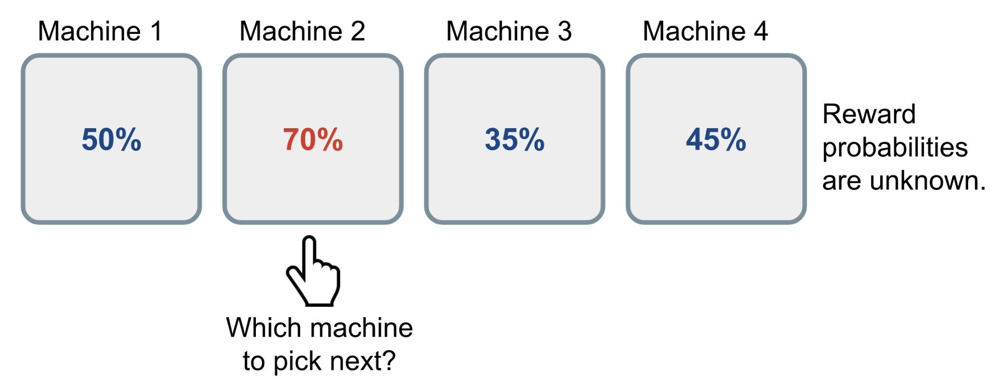
A naive approach is to keep playing a single machine for many, many rounds, eventually estimating its “true” reward probability via the law of large numbers. However, this is highly inefficient and certainly does not guarantee the best long-term reward.

Definition

Now, let’s define the problem more formally.

A Bernoulli multi-armed bandit can be described as a tuple of $\langle \mathcal{A}, \mathcal{R} \rangle$, where:

• We have $K$ machines with reward probabilities, $\{ \theta_1, \dots, \theta_K \}$.
• At each time step t, we take an action a on one slot machine and receive a reward r.
• $\mathcal{A}$ is a set of actions, each referring to interacting with one slot machine. The value of action a is the expected reward, $Q(a) = \mathbb{E} [r \vert a] = \theta$. If action $a_t$ at time step t selects the i-th machine, then $Q(a_t) = \theta_i$.
• $\mathcal{R}$ is a reward function. In the Bernoulli bandit setting, the reward r is observed in a stochastic manner. At time step t, $r_t = \mathcal{R}(a_t)$ may return reward 1 with probability $Q(a_t)$, and 0 otherwise.

This is a simplified version of a Markov decision process, since there is no state $\mathcal{S}$.

The objective is to maximize the cumulative reward $\sum_{t=1}^T r_t$. If we know the optimal action with the highest reward, then this objective is equivalent to minimizing the potential regret (or loss) incurred by not selecting the optimal action.

The optimal reward probability $\theta^{*}$ of the optimal action $a^{*}$ is:

Our loss function is the total regret from failing to select the optimal action up to time step T:

Bandit Strategies

Depending on how exploration is handled, there are several approaches to solving the multi-armed bandit problem.

• No exploration: the most naive approach, and a poor one.
• Exploration at random
• Exploration performed intelligently, with a preference for uncertainty

ε-Greedy Algorithm

The ε-greedy algorithm selects the best known action most of the time, while occasionally exploring by choosing an action at random. The action value is estimated from past experience by averaging the rewards observed for the target action a so far (up to the current time step t):

where $\mathbb{1}$ is a binary indicator function, and $N_t(a)$ is the number of times action a has been selected so far, $N_t(a) = \sum_{\tau=1}^t \mathbb{1}[a_\tau = a]$.

Under ε-greedy, with a small probability $\epsilon$ we take a random action; otherwise (which should occur most of the time, with probability 1-$\epsilon$), we choose the best action learned so far: $\hat{a}^{*}_t = \arg\max_{a \in \mathcal{A}} \hat{Q}_t(a)$.

See my toy implementation here.

Upper Confidence Bounds

Random exploration enables us to try options we do not yet understand well. However, because it is random, we may repeatedly explore an action that we have already identified as poor (unlucky!). To reduce such inefficient exploration, one approach is to decay ε over time. Another approach is to be optimistic about actions with high uncertainty, prioritizing those for which we do not yet have a confident estimate. Put differently, we favor exploring actions that have strong potential to be optimal.

The Upper Confidence Bounds (UCB) algorithm quantifies this potential using an upper confidence bound on the reward value, $\hat{U}_t(a)$, such that the true value lies below it with probability $Q(a) \leq \hat{Q}_t(a) + \hat{U}_t(a)$ (with high probability). The upper bound $\hat{U}_t(a)$ is a function of $N_t(a)$; with more trials $N_t(a)$, the bound should shrink, yielding a smaller $\hat{U}_t(a)$.

In the UCB algorithm, we always choose the greedy action that maximizes the upper confidence bound:

The remaining question is how to estimate the upper confidence bound.

Hoeffding’s Inequality

If we do not want to impose any prior assumptions about the distribution’s shape, we can use “Hoeffding’s Inequality”, a theorem that applies to any bounded distribution.

Let $X_1, \dots, X_t$ be i.i.d. (independent and identically distributed) random variables, all bounded within [0, 1]. The sample mean is $\overline{X}_t = \frac{1}{t}\sum_{\tau=1}^t X_\tau$. Then for $u > 0$, we have:

For a target action $a$, consider:

• $r_t(a)$ as the random variables,
• $Q(a)$ as the true mean,
• $\hat{Q}_t(a)$ as the sample mean,
• And $u$ as the upper confidence bound, $u = U_t(a)$

Then,

We want to choose a bound such that, with high probability, the true mean is below the sample mean plus the upper confidence bound. Therefore, $e^{-2t U_t(a)^2}$ should be small. Suppose we are comfortable with a tiny threshold p:

UCB1

One heuristic is to decrease the threshold p over time, because with more observed rewards we want a more confident bound. By setting $p=t^{-4}$, we obtain the UCB1 algorithm:

Bayesian UCB

In the UCB and UCB1 algorithms, we do not assume a prior for the reward distribution, so we rely on Hoeffding’s Inequality to obtain a very general bound estimate. If we know the distribution in advance, we can often construct a tighter bound estimate.

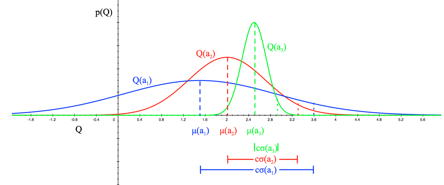
For example, if we expect each slot machine’s mean reward to be Gaussian, as in Fig 2, we can define the upper bound as a 95% confidence interval by setting $\hat{U}_t(a)$ to be twice the standard deviation.

See my toy implementations of UCB1 and Bayesian UCB with a Beta prior on θ.

Thompson Sampling

Thompson sampling is based on a simple idea, and it performs very well for the multi-armed bandit problem.

At each time step, we aim to select action a according to the probability that a is optimal:

where $\pi(a ; \vert ; h_t)$ is the probability of taking action a given the history $h_t$.

For the Bernoulli bandit, it is natural to assume that $Q(a)$ follows a Beta distribution, since $Q(a)$ is effectively the success probability θ in a Bernoulli distribution. The value of $\text{Beta}(\alpha, \beta)$ lies in the interval [0, 1]. The parameters α and β correspond to the counts of successes and failures in receiving a reward, respectively.

First, initialize the Beta parameters α and β for every action based on prior knowledge or belief. For example:

• α = 1 and β = 1; we expect a 50% reward probability, but we are not very confident.
• α = 1000 and β = 9000; we strongly believe the reward probability is 10%.

At each time t, we sample an expected reward $\tilde{Q}(a)$ from the prior distribution $\text{Beta}(\alpha_i, \beta_i)$ for every action. We then select the best action based on these samples: $a^{TS}_t = \arg\max_{a \in \mathcal{A}} \tilde{Q}(a)$. After observing the actual reward, we update the Beta distribution accordingly. This is Bayesian inference, computing the posterior from the prior and the likelihood of the observed data.

Thompson sampling implements probability matching. Because reward estimates $\tilde{Q}$ are drawn from posterior distributions, each probability corresponds to the probability that the associated action is optimal, conditioned on the observed history.

However, in many practical and complex settings, estimating posterior distributions from observed rewards via Bayesian inference can be computationally intractable. Thompson sampling can still be applied if we can approximate posterior distributions using methods such as Gibbs sampling, Laplace approximate, and the bootstraps. This tutorial offers a comprehensive review; I strongly recommend it if you want to learn more about Thompson sampling.

Case Study

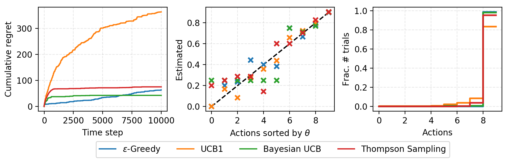
I implemented the algorithms above in lilianweng/multi-armed-bandit. A BernoulliBandit object can be created from a list of random or predefined reward probabilities. The bandit algorithms are implemented as subclasses of Solver, which take a Bandit object as the target problem. Cumulative regrets are tracked over time.

Summary

We need exploration because information has value. Regarding exploration strategies, we can choose to do no exploration and focus purely on short-term returns. Alternatively, we can explore randomly from time to time. Finally, we can go further by exploring selectively, favoring actions with higher uncertainty because they can provide greater information gain.

---

Cited as:

@article{weng2018bandit,
  title   = "The Multi-Armed Bandit Problem and Its Solutions",
  author  = "Weng, Lilian",
  journal = "lilianweng.github.io",
  year    = "2018",
  url     = "https://lilianweng.github.io/posts/2018-01-23-multi-armed-bandit/"
}

References

[1] CS229 Supplemental Lecture notes: Hoeffding’s inequality.

[2] RL Course by David Silver - Lecture 9: Exploration and Exploitation

[3] Olivier Chapelle and Lihong Li. “An empirical evaluation of thompson sampling.” NIPS. 2011.

[4] Russo, Daniel, et al. “A Tutorial on Thompson Sampling.” arXiv:1707.02038 (2017).