A (Long) Peek into Reinforcement Learning
[Updated on 2020-09-03: Revised the SARSA and Q-learning algorithms to make their differences more explicit. [Updated on 2021-09-19: Thanks to 爱吃猫的鱼, this post is now available in Chinese].
· 31 min read · Curated and presented by Arthur Sedek
[Updated on 2020-09-03: Updated the algorithm of SARSA and Q-learning so that the difference is more pronounced.
[Updated on 2021-09-19: Thanks to 爱吃猫的鱼, we have this post in Chinese].
Several major breakthroughs in Artificial Intelligence (AI) have occurred in recent years. AlphaGo defeated the top professional human player in the game of Go. Shortly afterward, the extended algorithm AlphaGo Zero defeated AlphaGo 100-0, without supervised learning from human knowledge. In DOTA2 1v1 competition, top professional players also lost to a bot developed by OpenAI. After seeing these results, it is difficult not to wonder about the mechanism behind such systems: Reinforcement Learning (RL). This post is written as a brief overview of the field. We will first define fundamental concepts and then move on to classic methods for solving RL problems. The goal is for this article to serve as a solid starting point for newcomers and to bridge into later study of cutting-edge research.
What is Reinforcement Learning?
Consider an agent operating in an unknown environment, where it can obtain rewards by interacting with that environment. The agent should select actions in order to maximize cumulative reward. In practice, this scenario may be a bot playing a game to achieve a high score, or a robot attempting to complete physical tasks with real objects, and it is not limited to these examples.
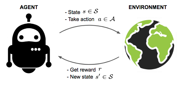
The objective of Reinforcement Learning (RL) is to learn an effective strategy for the agent through experimental trials and relatively simple feedback. With an optimal strategy, the agent can actively adapt to the environment in order to maximize future rewards.
Key Concepts
Next, we formally define a set of key concepts in RL.
An agent acts within an environment. The way the environment responds to actions is determined by a model, which we may or may not know. The agent can occupy one of many states ($s \in \mathcal{S}$) of the environment and can choose one of many actions ($a \in \mathcal{A}$) to move from one state to another. The resulting next state is governed by transition probabilities between states ($P$). After an action is taken, the environment emits a reward ($r \in \mathcal{R}$) as feedback.
The model specifies the reward function and the transition probabilities. Depending on whether we know the model, we distinguish two settings:
- Know the model: planning with perfect information; do model-based RL. When the environment is fully known, we can compute an optimal solution using Dynamic Programming (DP). Do you still remember “longest increasing subsequence” or “traveling salesmen problem” from your Algorithms 101 class? LOL. This is not the focus of this post though.
- Does not know the model: learning with incomplete information; do model-free RL or explicitly learn the model as part of the algorithm. Most of the material below focuses on the unknown-model setting.
The agent’s policy $\pi(s)$ provides guidance on which action is optimal in a given state, with the goal to maximize the total rewards. Each state is associated with a value function $V(s)$ that predicts the expected amount of future reward obtainable from that state when acting according to the corresponding policy. Put differently, the value function quantifies how good a state is. In reinforcement learning, both the policy and the value function are learning targets.
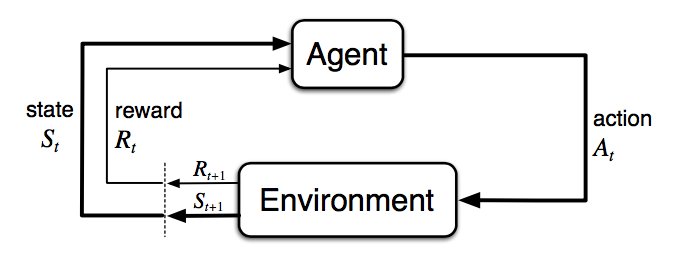
Agent-environment interaction unfolds over time as a sequence of actions and observed rewards, $t=1, 2, \dots, T$. Throughout this process, the agent accumulates knowledge about the environment, learns an optimal policy, and chooses which action to take next in order to learn the best policy efficiently. Let the state, action, and reward at time step t be $S_t$, $A_t$, and $R_t$, respectively. Then a single episode (also called a “trial” or “trajectory”) fully describes the interaction sequence, and the sequence ends at the terminal state $S_T$:
When exploring RL algorithms, you will frequently encounter these terms:
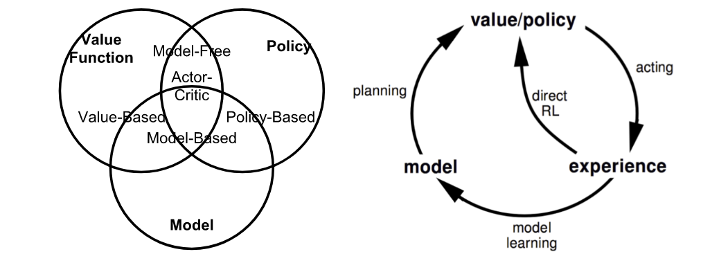
- Model-based: Depend on an environment model, either because it is known or because the algorithm explicitly learns it.
- Model-free: Do not rely on a model during learning.
- On-policy: Train using deterministic outcomes or samples generated by the target policy.
- Off-policy: Train on a distribution of transitions or episodes generated by a different behavior policy rather than by the target policy.
Model: Transition and Reward
The model describes the environment. With a model, we can learn or infer how the environment responds to the agent and how it provides feedback. The model comprises two primary components: the transition probability function $P$ and the reward function $R$.
Suppose that, in state s, we choose action a, arrive in next state s’, and receive reward r. This is a single transition step, represented by the tuple (s, a, s’, r).
The transition function P records the probability of moving from state s to s’ after taking action a and receiving reward r. We use $\mathbb{P}$ to denote “probability”.
Therefore, the state-transition function can be expressed as a function of $P(s’, r \vert s, a)$:
The reward function R predicts the next reward produced by taking an action:
Policy
A policy, as the agent’s behavior function $\pi$, specifies which action to take in state s. It maps a state s to an action a and may be deterministic or stochastic:
- Deterministic: $\pi(s) = a$.
- Stochastic: $\pi(a \vert s) = \mathbb{P}_\pi [A=a \vert S=s]$.
Value Function
A value function measures the quality of a state, or how rewarding a state or action is, by predicting future reward. The future reward, also called the return, is the sum of discounted rewards over time. Let us compute the return $G_t$ starting at time t:
The discount factor $\gamma \in [0, 1]$ penalizes future rewards for several reasons:
- Future rewards may be more uncertain (for example, in the stock market).
- Future rewards do not provide immediate benefit (for example, as human beings, we might prefer to have fun today rather than 5 years later ;)).
- Discounting offers mathematical convenience (for example, we do not need to track future steps forever to compute the return).
- It prevents us from having to worry about infinite loops in the state transition graph.
The state-value of a state s is the expected return when we are in this state at time t, $S_t = s$:
Similarly, the action-value (the “Q-value”; Q as “Quality” I believe?) for a state-action pair is defined as:
Additionally, because we follow the target policy $\pi$, we can use the probability distribution over actions together with Q-values to recover the state-value:
The action advantage function (the “A-value”) is the difference between action-value and state-value:
Optimal Value and Policy
The optimal value function yields the maximum return:
The optimal policy achieves the optimal value functions:
And of course, we have $V_{\pi_{*}}(s)=V_{*}(s)$ and $Q_{\pi_{*}}(s, a) = Q_{*}(s, a)$.
Markov Decision Processes
More formally, nearly all RL problems can be formulated as Markov Decision Processes (MDPs). Every state in an MDP satisfies the Markov property, meaning that the future depends only on the current state and not on the history:
Equivalently, given the present, the future and the past are conditionally independent, because the current state captures all the statistics required to determine what happens next.
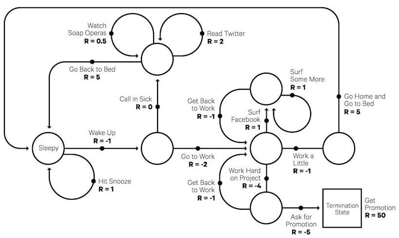
A Markov deicison process includes five elements $\mathcal{M} = \langle \mathcal{S}, \mathcal{A}, P, R, \gamma \rangle$. These symbols have the same meanings as the key concepts in the previous section and align well with standard RL problem settings:
- $\mathcal{S}$ - a set of states;
- $\mathcal{A}$ - a set of actions;
- $P$ - transition probability function;
- $R$ - reward function;
- $\gamma$ - discounting factor for future rewards. In an unknown environment, we do not have perfect knowledge about $P$ and $R$.
Bellman Equations
Bellman equations are a set of relations that decompose the value function into the immediate reward plus discounted future value.
Similarly, for the Q-value:
Bellman Expectation Equations
The recursive update can be further expanded into equations involving both the state-value and action-value functions. As we move forward through time steps, we alternately expand V and Q by following the policy $\pi$.
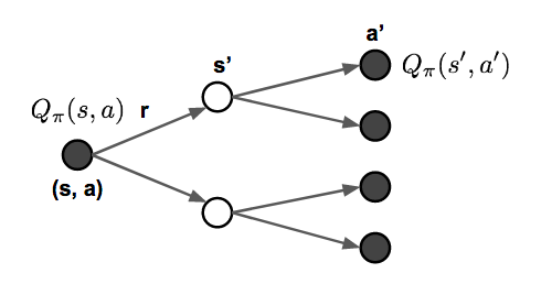
Bellman Optimality Equations
If our objective is only the optimal values, rather than an expectation under a particular policy, we can directly take the maximum return in the alternating updates, without referring to any policy. RECAP: the optimal values $V_*$ and $Q_*$ are the best returns achievable, defined here.
As expected, these equations closely resemble the Bellman expectation equations.
When we have complete information about the environment, this becomes a planning problem that DP can solve. However, in most cases we do not know $P_{ss’}^a$ or $R(s, a)$, so we cannot solve MDPs by directly applying Bellmen equations. Still, this framework provides the theoretical foundation for many RL algorithms.
Common Approaches
Next, we walk through major approaches and classic algorithms for solving RL problems. In future posts, I plan to explore each approach in more depth.
Dynamic Programming
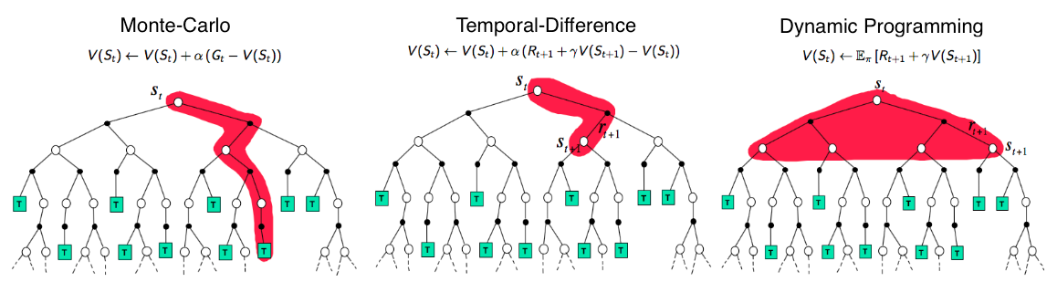
When the model is fully known, we can follow Bellman equations and use Dynamic Programming (DP) to iteratively evaluate value functions and improve the policy.
Policy Evaluation
Policy Evaluation computes the state-value $V_\pi$ for a fixed policy $\pi$:
Policy Improvement
Given the value functions, Policy Improvement constructs an improved policy $\pi’ \geq \pi$ by acting greedily.
Policy Iteration
The Generalized Policy Iteration (GPI) algorithm is an iterative procedure for policy improvement that combines policy evaluation with policy improvement.
In GPI, the value function is repeatedly approximated to move closer to the true value under the current policy. At the same time, the policy is repeatedly improved to move toward optimality. This policy iteration procedure works and always converges to the optimum, but why does this happen?
Suppose we start with a policy $\pi$ and then construct an improved policy $\pi’$ by selecting actions greedily, $\pi’(s) = \arg\max_{a \in \mathcal{A}} Q_\pi(s, a)$. The value under this improved $\pi’$ is guaranteed to be better because:
Monte-Carlo Methods
First, recall that $V(s) = \mathbb{E}[ G_t \vert S_t=s]$. Monte-Carlo (MC) methods rely on a straightforward idea: they learn from episodes of raw experience without modeling environment dynamics, and they use the observed mean return as an approximation to the expected return. To compute the empirical return $G_t$, MC methods must learn from complete episodes $S_1, A_1, R_2, \dots, S_T$ to compute $G_t = \sum_{k=0}^{T-t-1} \gamma^k R_{t+k+1}$, and all episodes must eventually terminate.
The empirical mean return for state s is:
where $\mathbb{1}[S_t = s]$ is a binary indicator function. We can count a visit to state s every time it occurs, allowing multiple visits to the same state within an episode (“every-visit”), or we can count only the first time the state is encountered in an episode (“first-visit”). The same approximation extends naturally to action-value functions by counting state-action pairs (s, a).
To learn the optimal policy with MC methods, we iterate using an approach similar in spirit to GPI.
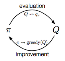
- Greedily improve the policy with respect to the current value function: $\pi(s) = \arg\max_{a \in \mathcal{A}} Q(s, a)$.
- Using the updated policy $\pi$, generate a new episode (that is, algorithms such as ε-greedy help balance exploitation and exploration).
- Estimate Q from the new episode: $q_\pi(s, a) = \frac{\sum_{t=1}^T \big( \mathbb{1}[S_t = s, A_t = a] \sum_{k=0}^{T-t-1} \gamma^k R_{t+k+1} \big)}{\sum_{t=1}^T \mathbb{1}[S_t = s, A_t = a]}$
Temporal-Difference Learning
Like Monte Carlo methods, Temporal-Difference (TD) learning is model-free and learns from episodes of experience. However, TD learning can also learn from incomplete episodes, so we do not need to follow an episode all the way to termination. TD learning is so central that Sutton & Barto (2017), in their RL book, describe it as “one idea … central and novel to reinforcement learning”.
Bootstrapping
TD methods update targets using existing estimates, rather than depending only on realized rewards and full returns as in Monte Carlo (MC) methods. This mechanism is called bootstrapping.
Value Estimation
The core idea in TD learning is to move the value function $V(S_t)$ toward an estimated return $R_{t+1} + \gamma V(S_{t+1})$ (the “TD target”). The learning-rate hyperparameter α determines the size of each update:
Similarly, for action-value estimation:
Next, we turn to the more interesting part: learning an optimal policy with TD learning (that is, “TD control”). Many well-known classic algorithms appear in this section.
SARSA: On-Policy TD control
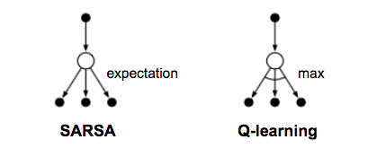
“SARSA” refers to updating the Q-value by following a sequence of $\dots, S_t, A_t, R_{t+1}, S_{t+1}, A_{t+1}, \dots$. The idea follows the same route as GPI. Within a single episode, the procedure is:
- Initialize $t=0$.
- Begin at $S_0$ and choose action $A_0 = \arg\max_{a \in \mathcal{A}} Q(S_0, a)$, where $\epsilon$-greedy is commonly used.
- At time $t$, after taking action $A_t$, observe reward $R_{t+1}$ and transition to the next state $S_{t+1}$.
- Select the next action using the same approach as in step 2: $A_{t+1} = \arg\max_{a \in \mathcal{A}} Q(S_{t+1}, a)$.
- Update the Q-value function: $ Q(S_t, A_t) \leftarrow Q(S_t, A_t) + \alpha (R_{t+1} + \gamma Q(S_{t+1}, A_{t+1}) - Q(S_t, A_t)) $.
- Set $t = t+1$ and repeat from step 3.
At each SARSA step, the next action must be selected according to the current policy.
Q-Learning: Off-policy TD control
The development of Q-learning (Watkins & Dayan, 1992) was a major breakthrough in the early days of Reinforcement Learning. Within one episode, it proceeds as follows:
- Initialize $t=0$.
- Start from $S_0$.
- At time step $t$, select an action according to the Q values, $A_t = \arg\max_{a \in \mathcal{A}} Q(S_t, a)$, and $\epsilon$-greedy is commonly applied.
- After taking action $A_t$, observe reward $R_{t+1}$ and transition to the next state $S_{t+1}$.
- Update the Q-value function: $Q(S_t, A_t) \leftarrow Q(S_t, A_t) + \alpha (R_{t+1} + \gamma \max_{a \in \mathcal{A}} Q(S_{t+1}, a) - Q(S_t, A_t))$.
- $t = t+1$ and repeat from step 3.
The key difference from SARSA is that Q-learning does not follow the current policy to choose the second action $A_{t+1}$. Instead, it estimates $Q^*$ using the best Q values; which action (denoted as $a^*$) achieves this maximum is irrelevant. As a result, in the next step Q-learning may not follow $a^*$.
Deep Q-Network
In principle, Q-learning can store $Q_*(.)$ for every state-action pair, similar to maintaining an enormous table. In practice, this quickly becomes computationally infeasible as state and action spaces grow. Consequently, Q values are often approximated with a function (that is, a machine learning model), an approach known as function approximation. For example, if we use a function parameterized by $\theta$ to compute Q values, we can denote the Q function as $Q(s, a; \theta)$.
Unfortunately, Q-learning can become unstable or even diverge when it is combined with a nonlinear Q-value function approximation and bootstrapping (see Problems #2).
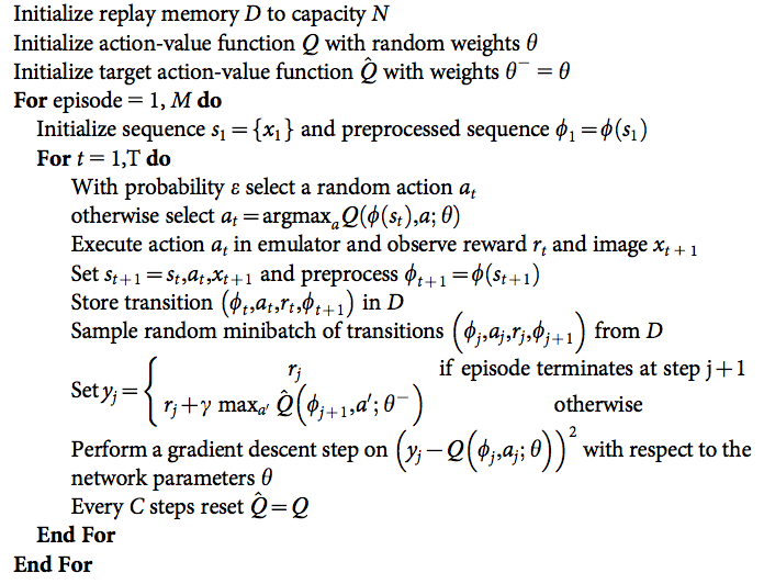
Deep Q-Network (“DQN”; Mnih et al. 2015) aims to substantially improve and stabilize Q-learning training through two key mechanisms:
- Experience Replay: All episode steps $e_t = (S_t, A_t, R_t, S_{t+1})$ are stored in a replay memory $D_t = \{ e_1, \dots, e_t \}$. $D_t$ contains experience tuples spanning many episodes. During Q-learning updates, samples are drawn uniformly at random from the replay memory, so a given sample can be reused multiple times. Experience replay improves data efficiency, breaks correlations in observation sequences, and smooths changes in the data distribution.
- Periodically Updated Target: Q is optimized toward target values that are updated only periodically. Every C steps (C is a hyperparameter), the Q network is cloned, and the clone is held fixed as the optimization target. This change stabilizes training by mitigating short-term oscillations.
The loss function is:
where $U(D)$ is a uniform distribution over the replay memory D; $\theta^{-}$ denotes the parameters of the frozen target Q-network.
Additionally, it has been found helpful to clip the error term to the range [-1, 1]. (I always have mixed feelings about parameter clipping: many studies show it works empirically, but it also makes the math less elegant. :/)
Many extensions of DQN improve on the original design, such as DQN with a dueling architecture (Wang et al. 2016), which estimates the state-value function V(s) and the advantage function A(s, a) using shared network parameters.
Combining TD and MC Learning
In the earlier section discussion of TD value estimation, the TD target looks only one step ahead along the action chain. This can be extended naturally to incorporate multiple steps when estimating the return.
Let the n-step estimated return be $G_t^{(n)}, n=1, \dots, \infty$; then:
| $n$ | $G_t$ | Notes |
|---|---|---|
| $n=1$ | $G_t^{(1)} = R_{t+1} + \gamma V(S_{t+1})$ | TD learning |
| $n=2$ | $G_t^{(2)} = R_{t+1} + \gamma R_{t+2} + \gamma^2 V(S_{t+2})$ | |
| … | ||
| $n=n$ | $ G_t^{(n)} = R_{t+1} + \gamma R_{t+2} + \dots + \gamma^{n-1} R_{t+n} + \gamma^n V(S_{t+n}) $ | |
| … | ||
| $n=\infty$ | $G_t^{(\infty)} = R_{t+1} + \gamma R_{t+2} + \dots + \gamma^{T-t-1} R_T + \gamma^{T-t} V(S_T) $ | MC estimation |
The generalized n-step TD method retains the same update form for the value function:
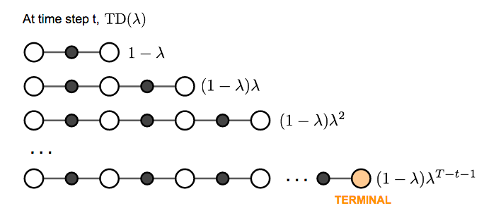
In TD learning, we can choose any $n$ we want. The question then becomes: what is the best $n$? Which $G_t^{(n)}$ yields the best approximation of the return? A common and effective solution is to use a weighted sum over all possible n-step TD targets, rather than selecting a single “best” n. The weights decay by a factor λ with n, $\lambda^{n-1}$. The intuition mirrors why: when computing returns, we discount future rewards because the further into the future we look, the less confident we are. To ensure the total weight (as n → ∞) sums to 1, we multiply each weight by (1-λ), because:
This weighted combination of n-step returns is the λ-return $G_t^{\lambda} = (1-\lambda) \sum_{n=1}^{\infty} \lambda^{n-1} G_t^{(n)}$. TD learning that uses the λ-return for value updates is denoted TD(λ). The original method introduced above corresponds to TD(0).
Policy Gradient
All methods introduced above learn a state-value or action-value function and then select actions accordingly. In contrast, Policy Gradient methods learn the policy directly via a parameterized function with respect to $\theta$, $\pi(a \vert s; \theta)$. Define the reward function (the opposite of a loss function) as expected return, and train the algorithm to maximize this reward function. My next post explains why the policy gradient theorem holds (including a proof) and introduces a number of policy gradient algorithms.
In discrete space:
where $S_1$ is the initial starting state.
Or in continuous space:
where $d_{\pi_\theta}(s)$ is the stationary distribution of the Markov chain for $\pi_\theta$. If the definition of “stationary distribution” is unfamiliar, see reference.
Using gradient ascent, we can search for the θ that yields the highest return. It is natural to expect that policy-based methods are more useful in continuous spaces: because there are infinitely many actions and/or states, value-based approaches require estimating values over an unbounded domain and therefore are computationally much more expensive.
Policy Gradient Theorem
We can compute the gradient numerically by perturbing θ by a small ε in the k-th dimension. This works even when $J(\theta)$ is not differentiable (nice!), but it is, unsurprisingly, very slow.
Or we can compute it analytically:
In fact, there is strong theoretical justification for replacing $d(.)$ with $d_\pi(.)$:
See Sec 13.1 in Sutton & Barto (2017) for the reasoning.
Then,
This result is called the “Policy Gradient Theorem,” and it provides the theoretical basis for many policy gradient algorithms:
REINFORCE
REINFORCE, also called the Monte Carlo policy gradient method, uses $Q_\pi(s, a)$, a return estimate from MC methods based on episode samples, to update the policy parameters $\theta$.
A widely used REINFORCE variant subtracts a baseline from the return $G_t$ to reduce the variance of the gradient estimate while leaving the bias unchanged. For example, a common baseline is the state value, in which case the gradient ascent update uses $A(s, a) = Q(s, a) - V(s)$.
- Initialize θ randomly.
- Generate one episode $S_1, A_1, R_2, S_2, A_2, \dots, S_T$.
- For t=1, 2, … , T:
- Estimate the return G_t from time step t onward.
- $\theta \leftarrow \theta + \alpha \gamma^t G_t \nabla \ln \pi(A_t \vert S_t, \theta)$.
Actor-Critic
When we learn a value function in addition to the policy, we obtain the Actor-Critic algorithm.
- Critic: updates value function parameters w; depending on the specific algorithm, it can be an action-value $Q(a \vert s; w)$ or a state-value $V(s; w)$.
- Actor: updates policy parameters θ in the direction recommended by the critic, $\pi(a \vert s; \theta)$.
Below is an example of how an action-value actor-critic algorithm operates.
- Initialize s, θ, and w randomly; sample $a \sim \pi(a \vert s; \theta)$.
- For t = 1… T:
- Sample reward $r_t \sim R(s, a)$ and next state $s’ \sim P(s’ \vert s, a)$.
- Then sample the next action $a’ \sim \pi(s’, a’; \theta)$.
- Update policy parameters: $\theta \leftarrow \theta + \alpha_\theta Q(s, a; w) \nabla_\theta \ln \pi(a \vert s; \theta)$.
- Compute the correction for the action value at time t:
$G_{t:t+1} = r_t + \gamma Q(s’, a’; w) - Q(s, a; w)$
and use it to update value function parameters:
$w \leftarrow w + \alpha_w G_{t:t+1} \nabla_w Q(s, a; w) $. - Update $a \leftarrow a’$ and $s \leftarrow s’$.
$\alpha_\theta$ and $\alpha_w$ are the learning rates for updating the policy and value-function parameters, respectively.
A3C
Asynchronous Advantage Actor-Critic (Mnih et al., 2016), abbreviated A3C, is a classic policy gradient method with a particular emphasis on parallel training.
In A3C, critics learn the state-value function $V(s; w)$, while multiple actors train in parallel and periodically synchronize with global parameters. Consequently, A3C is naturally suited for parallel training, for example, on a single machine with a multi-core CPU.
The state-value loss minimizes the mean squared error $\mathcal{J}_v (w) = (G_t - V(s; w))^2$, and gradient descent is used to obtain the optimal w. This state-value function serves as the baseline for the policy gradient update.
Algorithm outline:
- Maintain global parameters θ and w, and thread-specific parameters θ’ and w'.
- Initialize the time step t = 1.
- While T <= T_MAX:
- Reset gradients: dθ = 0 and dw = 0.
- Synchronize thread-specific parameters with the global ones: θ’ = θ and w’ = w.
- $t_\text{start}$ = t and get $s_t$.
- While ($s_t \neq \text{TERMINAL}$) and ($t - t_\text{start} <= t_\text{max}$):
- Select action $a_t \sim \pi(a_t \vert s_t; \theta’)$, then receive reward $r_t$ and new state $s_{t+1}$.
- Update t = t + 1 and T = T + 1.
- Initialize the variable holding the return estimate $R = \begin{cases} 0 & \text{if } s_t \text{ is TERMINAL} \ V(s_t; w’) & \text{otherwise} \end{cases}$.
- For $i = t-1, \dots, t_\text{start}$:
- $R \leftarrow r_i + \gamma R$; here R is an MC estimate of $G_i$.
- Accumulate gradients with respect to θ’: $d\theta \leftarrow d\theta + \nabla_{\theta’} \log \pi(a_i \vert s_i; \theta’)(R - V(s_i; w’))$;
Accumulate gradients with respect to w’: $dw \leftarrow dw + \nabla_{w’} (R - V(s_i; w’))^2$.
- Synchronously update θ using dθ, and update w using dw.
A3C enables parallelism across multiple training agents. The gradient accumulation step (6.2) can be viewed as a reformulation of minibatch-based stochastic gradient updates: each thread independently nudges w or θ slightly in its own gradient direction.
Evolution Strategies
Evolution Strategies (ES) is a model-agnostic optimization approach. It searches for an optimal solution by imitating Darwin’s theory of evolution by natural selection. ES requires two prerequisites: (1) solutions must be able to interact with the environment to test whether they solve the problem; (2) we must be able to compute a fitness score for each solution. We do not need to know the environment configuration in order to solve the task.
Assume we begin with a population of random solutions. Each candidate can interact with the environment, and only those with high fitness scores survive (only the fittest can survive in a competition for limited resources). A new generation is produced by recombining the configurations (gene mutation) of the high-fitness survivors. This loop repeats until the solutions are sufficiently strong.
Unlike the MDP-based approaches described above, ES learns the policy parameters $\theta$ directly, without value approximation. Assume the distribution over parameters $\theta$ is an isotropic multivariate Gaussian with mean $\mu$ and fixed covariance $\sigma^2I$. The gradient of $F(\theta)$ is:
We can rewrite the expression in terms of a “mean” parameter $\theta$ (distinct from $\theta$ above; this $\theta$ is the base gene for subsequent mutation), $\epsilon \sim N(0, I)$, and thus $\theta + \epsilon \sigma \sim N(\theta, \sigma^2)$. $\epsilon$ controls the magnitude of Gaussian noise added to generate mutations:
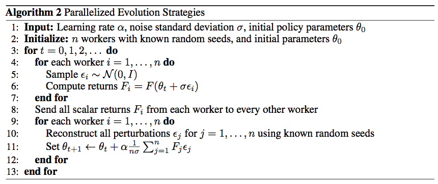
As a black-box optimization method, ES provides another approach to RL problems (In my original writing, I used the phrase “a nice alternative”; Seita pointed me to this discussion and thus I updated my wording.). It has several advantageous properties (Salimans et al., 2017) that keep it fast and straightforward to train:
- ES does not require value function approximation.
- ES does not perform gradient back-propagation.
- ES is invariant to delayed or long-term rewards.
- ES is highly parallelizable with minimal data communication.
Known Problems
Exploration-Exploitation Dilemma
The exploration versus exploitation dilemma is discussed in my earlier post. When an RL problem involves an unknown environment, this tradeoff is particularly critical for achieving strong performance: without sufficient exploration, we cannot learn the environment well enough; without sufficient exploitation, we cannot complete the reward optimization objective.
Different RL algorithms handle the balance between exploration and exploitation in different ways. In MC methods, Q-learning, or many on-policy algorithms, exploration is commonly implemented via ε-greedy. In ES, exploration is achieved through perturbations of the policy parameters. Keep this in mind when developing a new RL algorithm.
Deadly Triad Issue
We value the efficiency and flexibility of TD methods that rely on bootstrapping. However, when off-policy learning, nonlinear function approximation, and bootstrapping are combined within a single RL algorithm, training can become unstable and difficult to converge. This phenomenon is known as the deadly triad (Sutton & Barto, 2017). Many deep-learning-based architectures have been proposed to address this issue, including DQN, which stabilizes learning via experience replay and an occasionally frozen target network.
Case Study: AlphaGo Zero
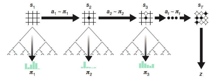
The game of Go has been an exceptionally difficult problem in Artificial Intelligence for decades, until recent years. AlphaGo and AlphaGo Zero are two programs developed by a DeepMind team. Both use deep Convolutional Neural Networks (CNN) and Monte Carlo Tree Search (MCTS), and both have been demonstrated to reach the level of professional human Go players. Unlike AlphaGo, which relied on supervised learning from expert human moves, AlphaGo Zero used only reinforcement learning and self-play, without human knowledge beyond the basic rules.
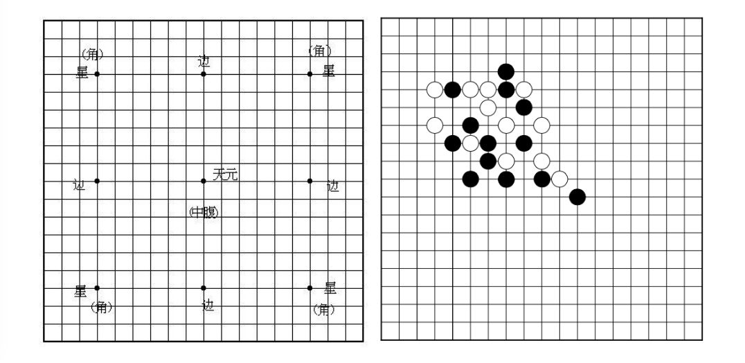
With the RL background above, we can now examine how AlphaGo Zero works. Its core component is a deep CNN over the game-board configuration (specifically, a ResNet with batch normalization and ReLU). The network produces two outputs:
- $s$: the board configuration represented as 19 x 19 x 17 stacked feature planes. There are 17 features per position: 8 past configurations (including the current one) for the current player, plus 8 past configurations for the opponent, plus 1 feature indicating color (1=black, 0=white). The color must be encoded explicitly because the network plays against itself, and the roles of current player and opponent alternate across steps.
- $p$: the probability of selecting a move among 19^2 + 1 candidates (19^2 board positions plus the pass action).
- $v$: the predicted probability of winning under the current configuration.
During self-play, MCTS further refines the action-probability distribution $\pi \sim p(.)$, and then action $a_t$ is sampled from this improved policy. The reward $z_t$ is binary, indicating whether the current player eventually wins the game. Each move yields an episode tuple $(s_t, \pi_t, z_t)$, which is stored in the replay memory. For space reasons, this post omits MCTS details; see the original paper if you would like more information.
The network is trained on samples from the replay memory by minimizing the loss:
where $c$ is a hyperparameter controlling the strength of the L2 penalty to prevent overfitting.
AlphaGo Zero simplified AlphaGo by eliminating supervised learning and combining separate policy and value networks into a single network. This design delivered significantly improved performance with substantially shorter training time. I strongly recommend reading two and papers side by side and comparing them, it is very fun.
I know this is a long read, but I hope it is worthwhile. If you notice mistakes and errors in this post, don’t hesitate to contact me at [lilian dot wengweng at gmail dot com]. See you in the next post! :)
Cited as:
@article{weng2018bandit,
  title   = "A (Long) Peek into Reinforcement Learning",
  author  = "Weng, Lilian",
  journal = "lilianweng.github.io",
  year    = "2018",
  url     = "https://lilianweng.github.io/posts/2018-02-19-rl-overview/"
}
References
[1] Yuxi Li. Deep reinforcement learning: An overview. arXiv preprint arXiv:1701.07274. 2017.
[2] Richard S. Sutton and Andrew G. Barto. Reinforcement Learning: An Introduction; 2nd Edition. 2017.
[3] Volodymyr Mnih, et al. Asynchronous methods for deep reinforcement learning. ICML. 2016.
[4] Tim Salimans, et al. Evolution strategies as a scalable alternative to reinforcement learning. arXiv preprint arXiv:1703.03864 (2017).
[5] David Silver, et al. Mastering the game of go without human knowledge. Nature 550.7676 (2017): 354.
[6] David Silver, et al. Mastering the game of Go with deep neural networks and tree search. Nature 529.7587 (2016): 484-489.
[7] Volodymyr Mnih, et al. Human-level control through deep reinforcement learning. Nature 518.7540 (2015): 529.
[8] Ziyu Wang, et al. Dueling network architectures for deep reinforcement learning. ICML. 2016.
[9] Reinforcement Learning lectures by David Silver on YouTube.
[10] OpenAI Blog: Evolution Strategies as a Scalable Alternative to Reinforcement Learning
[11] Frank Sehnke, et al. Parameter-exploring policy gradients. Neural Networks 23.4 (2010): 551-559.
[12] Csaba Szepesvári. Algorithms for reinforcement learning. 1st Edition. Synthesis lectures on artificial intelligence and machine learning 4.1 (2010): 1-103.
If you notice mistakes and errors in this post, please don’t hesitate to contact me at [lilian dot wengweng at gmail dot com] and I would be super happy to correct them right away!