Implementing Deep Reinforcement Learning Models with Tensorflow + OpenAI Gym
The complete implementation is available in lilianweng/deep-reinforcement-learning-gym. In the previous two posts, I introduced the algorithms behind a range of deep reinforcement learning models. Now it is time to get hands-on and apply those models in practice. This implementation is built using Tensorflow and the OpenAI Gym environment. The full version of the code used in this tutorial is available in [lilian/deep-reinforcement-learning-gym].
· 13 min read · Curated and presented by Arthur Sedek
The complete implementation is available at lilianweng/deep-reinforcement-learning-gym.
In the previous two posts, I introduced the algorithms behind many deep reinforcement learning models. Now it is time to move from theory to practice and implement these models in real-world code. The implementations will use Tensorflow and the OpenAI gym environment. The full version of the code for this tutorial is available at [lilian/deep-reinforcement-learning-gym].
Environment Setup
- Confirm that Homebrew is installed:
/usr/bin/ruby -e "$(curl -fsSL https://raw.githubusercontent.com/Homebrew/install/master/install)"
- I recommend starting a virtualenv for development. This makes it much easier to manage multiple projects with conflicting dependencies, for example, one project that runs on Python 2.7 while another requires Python 3.5+.
# Install python virtualenv
brew install pyenv-virtualenv
# Create a virtual environment of any name you like with Python 3.6.4 support
pyenv virtualenv 3.6.4 workspace
# Activate the virtualenv named "workspace"
pyenv activate workspace
[*] For each new installation step below, make sure you are working inside the virtualenv.
- Install OpenAI gym by following the instruction. For a minimal installation, run:
git clone https://github.com/openai/gym.git
cd gym
pip install -e .
If you want to experiment with Atari games or other advanced packages, continue by installing a few additional system packages.
brew install cmake boost boost-python sdl2 swig wget
For Atari, navigate to the gym directory and install the Atari dependencies with pip. This post can be helpful if you run into issues installing ALE (the arcade learning environment).
pip install -e '.[atari]'
- Finally, clone the “playground” code and install the required dependencies.
git clone [email protected]:lilianweng/deep-reinforcement-learning-gym.git
cd deep-reinforcement-learning-gym
pip install -e .  # install the "playground" project.
pip install -r requirements.txt  # install required packages.
Gym Environment
The OpenAI Gym toolkit offers a collection of physical simulation environments, games, and robot simulators that you can use to experiment with and build reinforcement learning agents. You can initialize an environment object with gym.make("{environment name}":
import gym
env = gym.make("MsPacman-v0")
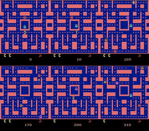
An environment’s action and observation formats are specified by env.action_space and env.observation_space, respectively.
Common Gym spaces types include:
gym.spaces.Discrete(n): discrete values ranging from 0 to n-1.gym.spaces.Box: a multi-dimensional vector of numeric values, where the lower and upper bounds of each dimension are defined byBox.lowandBox.high.
We interact with an environment primarily through two API calls:
ob = env.reset()
- Resets the environment to its initial configuration.
- Returns the initial observation.
ob_next, reward, done, info = env.step(action)
- Applies a single action to the environment, and the action must be compatible with
env.action_space. - Returns the next observation
ob_next(env.observation_space), a reward (float), adoneflag (bool), and additional metadata (dict). Ifdone=True, the episode has ended and the environment should be reset to begin again. Read more here.
Naive Q-Learning
Q-learning (Watkins & Dayan, 1992) learns the action value (the “Q-value”) and updates it according to the Bellman equation. The key idea is that, when estimating the next action, it does not follow the current policy. Instead, it independently selects the best Q value (the part in red).
In a naive implementation, the Q value for all (s, a) pairs can be stored directly in a dictionary. At this stage, no complex machine learning model is required.
from collections import defaultdict
Q = defaultdict(float)
gamma = 0.99  # Discounting factor
alpha = 0.5  # soft update param

env = gym.make("CartPole-v0")
actions = range(env.action_space)

def update_Q(s, r, a, s_next, done):
    max_q_next = max([Q[s_next, a] for a in actions])
    # Do not include the next state's value if currently at the terminal state.
    Q[s, a] += alpha * (r + gamma * max_q_next * (1.0 - done) - Q[s, a])
Most Gym environments have a multi-dimensional continuous observation space (gym.spaces.Box). To prevent the Q dictionary from exploding as it attempts to memorize an infinite number of keys, we apply a wrapper that discretizes the observation. The concept of wrappers is highly flexible, enabling customization of an environment’s observation, action, step function, and more. Regardless of how many wrappers are applied, env.unwrapped always returns the underlying original environment object.
import gym

class DiscretizedObservationWrapper(gym.ObservationWrapper):
    """This wrapper converts a Box observation into a single integer.
    """
    def __init__(self, env, n_bins=10, low=None, high=None):
        super().__init__(env)
        assert isinstance(env.observation_space, Box)

        low = self.observation_space.low if low is None else low
        high = self.observation_space.high if high is None else high

        self.n_bins = n_bins
        self.val_bins = [np.linspace(l, h, n_bins + 1) for l, h in
                         zip(low.flatten(), high.flatten())]
        self.observation_space = Discrete(n_bins ** low.flatten().shape[0])

    def _convert_to_one_number(self, digits):
        return sum([d * ((self.n_bins + 1) ** i) for i, d in enumerate(digits)])

    def observation(self, observation):
        digits = [np.digitize([x], bins)[0]
                  for x, bins in zip(observation.flatten(), self.val_bins)]
        return self._convert_to_one_number(digits)


env = DiscretizedObservationWrapper(
    env,
    n_bins=8,
    low=[-2.4, -2.0, -0.42, -3.5],
    high=[2.4, 2.0, 0.42, 3.5]
)
Next, we integrate environment interaction and update the Q function each time a new transition is produced. For action selection, we use ε-greedy to encourage exploration.
import gym
import numpy as np
n_steps = 100000
epsilon = 0.1  # 10% chances to apply a random action

def act(ob):
    if np.random.random() < epsilon:
        # action_space.sample() is a convenient function to get a random action
        # that is compatible with this given action space.
        return env.action_space.sample()

    # Pick the action with highest q value.
    qvals = {a: q[state, a] for a in actions}
    max_q = max(qvals.values())
    # In case multiple actions have the same maximum q value.
    actions_with_max_q = [a for a, q in qvals.items() if q == max_q]
    return np.random.choice(actions_with_max_q)

ob = env.reset()
rewards = []
reward = 0.0

for step in range(n_steps):
    a = act(ob)
    ob_next, r, done, _ = env.step(a)
    update_Q(ob, r, a, ob_next, done)
    reward += r
    if done:
        rewards.append(reward)
        reward = 0.0
        ob = env.reset()
    else:
        ob = ob_next
In practice, we often begin with a relatively high epsilon and then gradually reduce it during training, a process commonly called “epsilon annealing”. The full code for QLearningPolicy is available here.
Deep Q-Network
Deep Q-network is a foundational work that improves the stability and data efficiency of Q-learning when the Q value is approximated by a nonlinear function. Its two key components are experience replay and a separately updated target network.
The main loss function is:
The Q network may be implemented as a multi-layer dense neural network, a convolutional network, or a recurrent network, depending on the task. In the full implementation of the DQN policy, this choice is controlled by the model_type parameter, one of (“dense”, “conv”, “lstm”).
In the example below, I use a 2-layer fully connected neural network to learn Q values for the cart pole balancing task.
import gym
env = gym.make('CartPole-v1')
# The observation space is `Box(4,)`, a 4-element vector.
observation_size = env.observation_space.shape[0]
The helper function below is used to construct the networks:
import tensorflow as tf
def dense_nn(inputs, layers_sizes, scope_name):
    """Creates a densely connected multi-layer neural network.
    inputs: the input tensor
    layers_sizes (list<int>): defines the number of units in each layer. The output
        layer has the size layers_sizes[-1].
    """
    with tf.variable_scope(scope_name):
        for i, size in enumerate(layers_sizes):
            inputs = tf.layers.dense(
                inputs,
                size,
                # Add relu activation only for internal layers.
                activation=tf.nn.relu if i < len(layers_sizes) - 1 else None,
                kernel_initializer=tf.contrib.layers.xavier_initializer(),
                name=scope_name + '_l' + str(i)
            )
    return inputs
The Q-network and the target network are updated using batches of transitions (state, action, reward, state_next, done_flag). The input tensors are:
batch_size = 32  # A tunable hyperparameter.

states = tf.placeholder(tf.float32, shape=(batch_size, observation_size), name='state')
states_next = tf.placeholder(tf.float32, shape=(batch_size, observation_size), name='state_next')
actions = tf.placeholder(tf.int32, shape=(batch_size,), name='action')
rewards = tf.placeholder(tf.float32, shape=(batch_size,), name='reward')
done_flags = tf.placeholder(tf.float32, shape=(batch_size,), name='done')
We define two networks with identical structures. Both share the same architecture, taking state observations as inputs and producing Q values for all actions as outputs.
q = dense(states, [32, 32, 2], name='Q_primary')
q_target = dense(states_next, [32, 32, 2], name='Q_target')
The target network, “Q_target”, uses the states_next tensor as input, since its predictions are used to select the optimal next state in the Bellman equation.
# The prediction by the primary Q network for the actual actions.
action_one_hot = tf.one_hot(actions, act_size, 1.0, 0.0, name='action_one_hot')
pred = tf.reduce_sum(q * action_one_hot, reduction_indices=-1, name='q_acted')

# The optimization target defined by the Bellman equation and the target network.
max_q_next_by_target = tf.reduce_max(q_target, axis=-1)
y = rewards + (1. - done_flags) * gamma * max_q_next_by_target

# The loss measures the mean squared error between prediction and target.
loss = tf.reduce_mean(tf.square(pred - tf.stop_gradient(y)), name="loss_mse_train")
optimizer = tf.train.AdamOptimizer(0.001).minimize(loss, name="adam_optim")
Note that tf.stop_gradient() on the target y, because the target network must remain fixed during the gradient update that minimizes the loss.
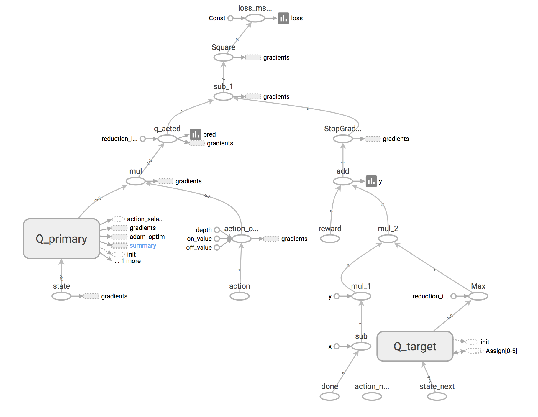
The target network is updated either by copying parameters from the primary Q network every C steps (“hard update”), or by Polyak averaging toward the primary network (“soft update”).
# Get all the variables in the Q primary network.
q_vars = tf.get_collection(tf.GraphKeys.GLOBAL_VARIABLES, scope="Q_primary")
# Get all the variables in the Q target network.
q_target_vars = tf.get_collection(tf.GraphKeys.GLOBAL_VARIABLES, scope="Q_target")
assert len(q_vars) == len(q_target_vars)

def update_target_q_net_hard():
    # Hard update
    sess.run([v_t.assign(v) for v_t, v in zip(q_target_vars, q_vars)])

def update_target_q_net_soft(tau=0.05):
    # Soft update: polyak averaging.
    sess.run([v_t.assign(v_t * (1. - tau) + v * tau) for v_t, v in zip(q_target_vars, q_vars)])
Double Q-Learning
Examining the standard Q target, $Y(s, a) = r + \gamma \max_{a’ \in \mathcal{A}} Q_\theta (s’, a’)$, it becomes clear that we use $Q_\theta$ to choose the best next action at state s’, and then evaluate that action using the value predicted by the same $Q_\theta$. This reinforcing two-step process can amplify overestimation (especially when values are already overestimated), which can in turn destabilize training. Double Q-learning (Hasselt, 2010) addresses this by decoupling action selection from action-value evaluation using two Q networks, $Q_1$ and $Q_2$: when $Q_1$ is updated, $Q_2$ selects the best next action, and vice versa.
To add double Q-learning to DQN, the smallest change (Hasselt, Guez, & Silver, 2016) is to use the primary Q network for action selection, while using the target network to estimate the corresponding action value:
In code, this requires introducing a new tensor that supplies the action selected by the primary Q network, along with a tensor operation that selects this action.
actions_next = tf.placeholder(tf.int32, shape=(None,), name='action_next')
actions_selected_by_q = tf.argmax(q, axis=-1, name='action_selected')
Accordingly, the prediction target y in the loss function becomes:
actions_next_flatten = actions_next + tf.range(0, batch_size) * q_target.shape[1]
max_q_next_target = tf.gather(tf.reshape(q_target, [-1]), actions_next_flatten)
y = rewards + (1. - done_flags) * gamma * max_q_next_by_target
Here, I used tf.gather() to select the action values of interest.
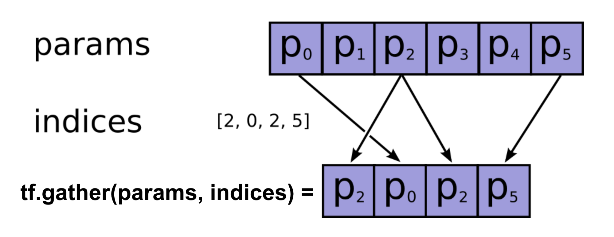
During rollout, we compute actions_next by feeding the next-state data into the actions_selected_by_q operation.
# batch_data is a dict with keys, ‘s', ‘a', ‘r', ‘s_next' and ‘done', containing a batch of transitions.
actions_next = sess.run(actions_selected_by_q, {states: batch_data['s_next']})
Dueling Q-Network
The dueling Q-network (Wang et al., 2016) uses an enhanced architecture in which the output layer splits into two heads: one predicts the state value V, and the other predicts the advantage A. The Q-value is then reconstructed as $Q(s, a) = V(s) + A(s, a)$.
To ensure the estimated advantage values sum to zero, $\sum_a A(s, a)\pi(a \vert s) = 0$, we subtract the mean value from the prediction.
The required code change is straightforward:
q_hidden = dense_nn(states, [32], name='Q_primary_hidden')
adv = dense_nn(q_hidden, [32, env.action_space.n], name='Q_primary_adv')
v = dense_nn(q_hidden, [32, 1], name='Q_primary_v')

# Average dueling
q = v + (adv - tf.reduce_mean(adv, reduction_indices=1, keepdims=True))
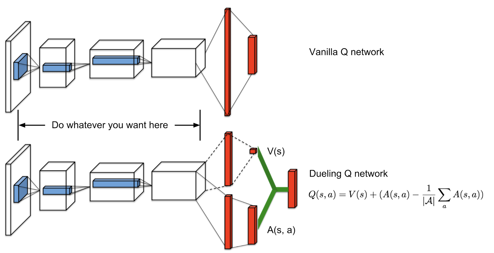
For the complete workflow, see the code.
Monte-Carlo Policy Gradient
I reviewed several widely used policy gradient methods in last post. Monte-Carlo policy gradient, also known as REINFORCE, is a classic on-policy approach that explicitly learns a policy model. It estimates returns from full on-policy trajectories and updates policy parameters via the policy gradient.
Returns are computed during rollouts and then provided to the TensorFlow graph as inputs.
# Inputs
states = tf.placeholder(tf.float32, shape=(None, obs_size), name='state')
actions = tf.placeholder(tf.int32, shape=(None,), name='action')
returns = tf.placeholder(tf.float32, shape=(None,), name='return')
We construct the policy network and update the policy parameters by minimizing the loss function, $\mathcal{L} = - (G_t - V(s)) \log \pi(a \vert s)$. tf.nn.sparse_softmax_cross_entropy_with_logits() requires the raw logits as inputs, rather than probabilities after softmax, which is why the policy network does not include a softmax layer at the top.
# Policy network
pi = dense_nn(states, [32, 32, env.action_space.n], name='pi_network')
sampled_actions = tf.squeeze(tf.multinomial(pi, 1))  # For sampling actions according to probabilities.

with tf.variable_scope('pi_optimize'):
    loss_pi = tf.reduce_mean(
        returns * tf.nn.sparse_softmax_cross_entropy_with_logits(
            logits=pi, labels=actions), name='loss_pi')
    optim_pi = tf.train.AdamOptimizer(0.001).minimize(loss_pi, name='adam_optim_pi')
During rollout, the return is computed as follows:
# env = gym.make(...)
# gamma = 0.99
# sess = tf.Session(...)

def act(ob):
    return sess.run(sampled_actions, {states: [ob]})

for _ in range(n_episodes):
    ob = env.reset()
    done = False

    obs = []
    actions = []
    rewards = []
    returns = []

    while not done:
        a = act(ob)
        new_ob, r, done, info = env.step(a)

        obs.append(ob)
        actions.append(a)
        rewards.append(r)
        ob = new_ob

    # Estimate returns backwards.
    return_so_far = 0.0
    for r in rewards[::-1]:
        return_so_far = gamma * return_so_far + r
        returns.append(return_so_far)

    returns = returns[::-1]

    # Update the policy network with the data from one episode.
    sess.run([optim_pi], feed_dict={
        states: np.array(obs),
        actions: np.array(actions),
        returns: np.array(returns),
    })
The full REINFORCE implementation is here.
Actor-Critic
The actor-critic algorithm learns two models simultaneously: an actor that learns the best policy, and a critic that estimates the state value.
- Initialize the actor network, $\pi(a \vert s)$, and the critic, $V(s)$
- Collect a new transition (s, a, r, s’): sample action $a \sim \pi(a \vert s)$ for the current state s, then observe the reward r and the next state s'.
- Compute the TD target during rollout, $G_t = r + \gamma V(s’)$, and the TD error, $\delta_t = r + \gamma V(s’) - V(s)$.
- Update the critic network by minimizing the critic loss: $L_c = (V(s) - G_t)$.
- Update the actor network by minimizing the actor loss: $L_a = - \delta_t \log \pi(a \vert s)$.
- Set s’ = s and repeat steps 2.-5.
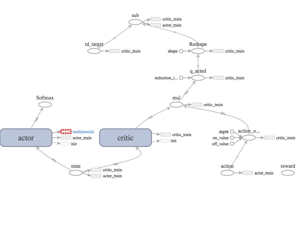
Overall, the implementation closely resembles REINFORCE, with the addition of a critic network. The full implementation is here.
# Inputs
states = tf.placeholder(tf.float32, shape=(None, observation_size), name='state')
actions = tf.placeholder(tf.int32, shape=(None,), name='action')
td_targets = tf.placeholder(tf.float32, shape=(None,), name='td_target')

# Actor: action probabilities
actor = dense_nn(states, [32, 32, env.action_space.n], name='actor')

# Critic: action value (Q-value)
critic = dense_nn(states, [32, 32, 1], name='critic')

action_ohe = tf.one_hot(actions, act_size, 1.0, 0.0, name='action_one_hot')
pred_value = tf.reduce_sum(critic * action_ohe, reduction_indices=-1, name='q_acted')
td_errors = td_targets - tf.reshape(pred_value, [-1])

with tf.variable_scope('critic_train'):
    loss_c = tf.reduce_mean(tf.square(td_errors))
    optim_c = tf.train.AdamOptimizer(0.01).minimize(loss_c)

with tf.variable_scope('actor_train'):
    loss_a = tf.reduce_mean(
        tf.stop_gradient(td_errors) * tf.nn.sparse_softmax_cross_entropy_with_logits(
            logits=actor, labels=actions),
        name='loss_actor')
    optim_a = tf.train.AdamOptimizer(0.01).minimize(loss_a)

train_ops = [optim_c, optim_a]
The TensorBoard graph is consistently useful:
References
[2] Christopher JCH Watkins, and Peter Dayan. “Q-learning.” Machine learning 8.3-4 (1992): 279-292.
[3] Hado Van Hasselt, Arthur Guez, and David Silver. “Deep Reinforcement Learning with Double Q-Learning.” AAAI. Vol. 16. 2016.
[4] Hado van Hasselt. “Double Q-learning.” NIPS, 23:2613–2621, 2010.
[5] Ziyu Wang, et al. Dueling network architectures for deep reinforcement learning. ICML. 2016.