From Autoencoder to Beta-VAE
[Updated on 2019-07-18: add a section on VQ-VAE & VQ-VAE-2.] [Updated on 2019-07-26: add a section on TD-VAE.] The autoencoder was introduced as a neural network approach for reconstructing high-dimensional data by passing inputs through a narrow bottleneck layer positioned midway through the model (oops, this is probably not true for Variational Autoencoder, and we will investigate it in details in later sections). One useful side effect is dimensionality reduction: the bottleneck layer learns a compressed latent encoding. This low-dimensional representation can serve as an embedding vector in a range of applications (i.e. search), support data compression, or expose the underlying generative factors in the data.
· 21 min read · Curated and presented by Arthur Sedek
[Updated on 2019-07-18: add a section on VQ-VAE & VQ-VAE-2.]
[Updated on 2019-07-26: add a section on TD-VAE.]
An autoencoder is intended to reconstruct high-dimensional data using a neural network with a narrow bottleneck layer in the middle (oops, this is probably not true for Variational Autoencoder, and we will investigate it in details in later sections). A helpful byproduct is dimensionality reduction: the bottleneck layer learns a compressed latent encoding. This low-dimensional representation can serve as an embedding vector in many applications (i.e. search), support data compression, or expose underlying generative factors in the data.
Notation
| Symbol | Mean |
|---|---|
| $\mathcal{D}$ | The dataset, $\mathcal{D} = \{ \mathbf{x}^{(1)}, \mathbf{x}^{(2)}, \dots, \mathbf{x}^{(n)} \}$, contains $n$ data samples; $\vert\mathcal{D}\vert =n $. |
| $\mathbf{x}^{(i)}$ | Each data point is a vector of $d$ dimensions, $\mathbf{x}^{(i)} = [x^{(i)}_1, x^{(i)}_2, \dots, x^{(i)}_d]$. |
| $\mathbf{x}$ | One data sample from the dataset, $\mathbf{x} \in \mathcal{D}$. |
| $\mathbf{x}’$ | The reconstructed version of $\mathbf{x}$. |
| $\tilde{\mathbf{x}}$ | The corrupted version of $\mathbf{x}$. |
| $\mathbf{z}$ | The compressed code learned in the bottleneck layer. |
| $a_j^{(l)}$ | The activation function for the $j$-th neuron in the $l$-th hidden layer. |
| $g_{\phi}(.)$ | The encoding function parameterized by $\phi$. |
| $f_{\theta}(.)$ | The decoding function parameterized by $\theta$. |
| $q_{\phi}(\mathbf{z}\vert\mathbf{x})$ | Estimated posterior probability function, also known as probabilistic encoder. |
| $p_{\theta}(\mathbf{x}\vert\mathbf{z})$ | Likelihood of generating true data sample given the latent code, also known as probabilistic decoder. |
Autoencoder
An autoencoder is a neural network that is trained, in an unsupervised manner, to learn an identity function. Its goal is to reconstruct the original input while compressing information along the way, thereby discovering a more efficient, compact representation. The idea originated in the 1980s and was later popularized by the seminal work Hinton & Salakhutdinov, 2006.
An autoencoder comprises two networks:
- Encoder network: Maps the original high-dimensional input into a latent low-dimensional code. The input dimensionality is larger than the output dimensionality.
- Decoder network: Reconstructs the data from the code, typically using output layers that grow larger and larger.
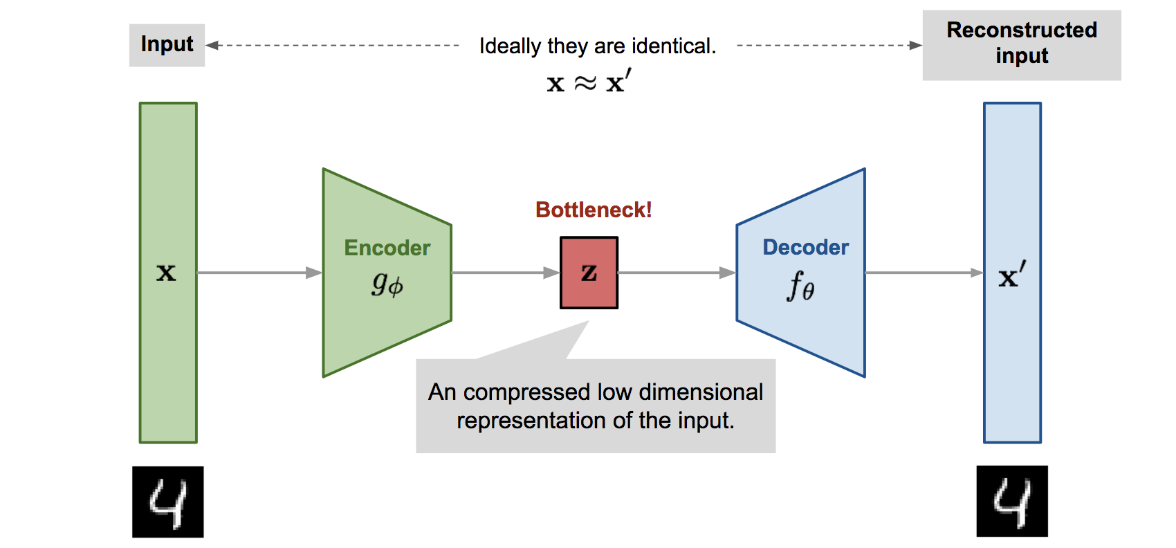
The encoder effectively performs the dimensionality reduction, similar to how we might apply Principal Component Analysis (PCA) or Matrix Factorization (MF). Additionally, the autoencoder is explicitly optimized to reconstruct the data from the code. A strong intermediate representation not only captures latent variables, but also supports a complete decompression process.
The model includes an encoder function $g(.)$ parameterized by $\phi$ and a decoder function $f(.)$ parameterized by $\theta$. For an input $\mathbf{x}$, the low-dimensional code learned in the bottleneck layer is $\mathbf{z} = g_\phi(\mathbf{x})$, and the reconstructed input is $\mathbf{x}’ = f_\theta(g_\phi(\mathbf{x}))$.
The parameters $(\theta, \phi)$ are learned jointly so that the model outputs a reconstructed sample identical to the original input, $\mathbf{x} \approx f_\theta(g_\phi(\mathbf{x}))$, that is, it learns an identity function. Many metrics can quantify the difference between two vectors, for example, cross entropy when the activation function is sigmoid, or as simply as MSE loss:
Denoising Autoencoder
Because an autoencoder is trained to learn an identity function, there is a risk of “overfitting” when the network has more parameters than there are data points.
To reduce overfitting and improve robustness, the Denoising Autoencoder (Vincent et al. 2008) introduces a modification to the basic autoencoder. The input is partially corrupted by stochastically adding noise to, or masking, some values of the input vector, $\tilde{\mathbf{x}} \sim \mathcal{M}_\mathcal{D}(\tilde{\mathbf{x}} \vert \mathbf{x})$. The model is then trained to recover the original input (note: not the corrupted one).
where $\mathcal{M}_\mathcal{D}$ defines the mapping from the true data samples to the noisy or corrupted samples.
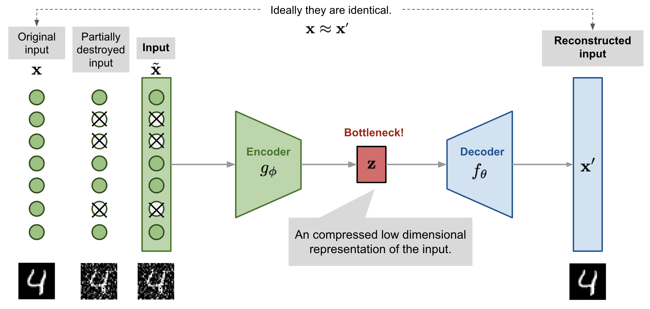
This design is motivated by the observation that humans can recognize an object or scene even when the view is partially occluded or corrupted. To “repair” the partially destroyed input, the denoising autoencoder must discover and capture relationships among input dimensions in order to infer the missing components.
For high-dimensional inputs with substantial redundancy, such as images, the model is more likely to rely on evidence combined across many input dimensions to recover the denoised version, rather than overfitting to any single dimension. This provides a strong basis for learning a robust latent representation.
The noise is governed by a stochastic mapping $\mathcal{M}_\mathcal{D}(\tilde{\mathbf{x}} \vert \mathbf{x})$, and it is not restricted to any particular corruption process (i.e. masking noise, Gaussian noise, salt-and-pepper noise, etc.). Naturally, the corruption process can incorporate prior knowledge
In experiments from the original DAE paper, noise is applied as follows: a fixed proportion of input dimensions are randomly selected, and their values are forced to 0. This sounds quite similar to dropout, right? However, the denoising autoencoder was proposed in 2008, four years before the dropout paper (Hinton, et al. 2012) ;)
**Stacked Denoising Autoencoder**: Before training deep neural networks became more practical, stacking denoising autoencoders was a common approach for building deep models ([Vincent et al., 2010](http://www.jmlr.org/papers/volume11/vincent10a/vincent10a.pdf)). Denoising autoencoders are trained one layer at a time. After one layer has been trained, it is provided with clean, uncorrupted inputs so it can learn the encoding for the next layer.
Sparse Autoencoder
A Sparse Autoencoder introduces a “sparsity” constraint on hidden-unit activations to reduce overfitting and improve robustness. It encourages only a small number of hidden units to be active at the same time, that is, each hidden neuron should be inactive most of the time.
Recall that common activation functions include sigmoid, tanh, relu, leaky relu, etc. A neuron is considered active when its value is close to 1, and inactive when its value is close to 0.
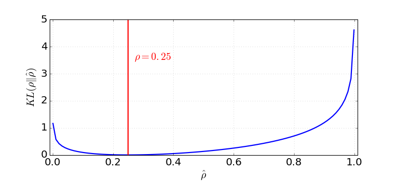
Assume there are $s_l$ neurons in the $l$-th hidden layer. The activation function for the $j$-th neuron in this layer is denoted $a^{(l)}_j(.)$, $j=1, \dots, s_l$. The expected activation frequency of this neuron $\hat{\rho}_j$ should be a small value $\rho$, called the sparsity parameter, and a common configuration is $\rho = 0.05$.
This constraint is implemented by adding a penalty term to the loss. The KL-divergence $D_\text{KL}$ measures the difference between two Bernoulli distributions, one with mean $\rho$ and the other with mean $\hat{\rho}_j^{(l)}$. The hyperparameter $\beta$ controls how strongly the sparsity penalty is applied.
$k$-Sparse Autoencoder
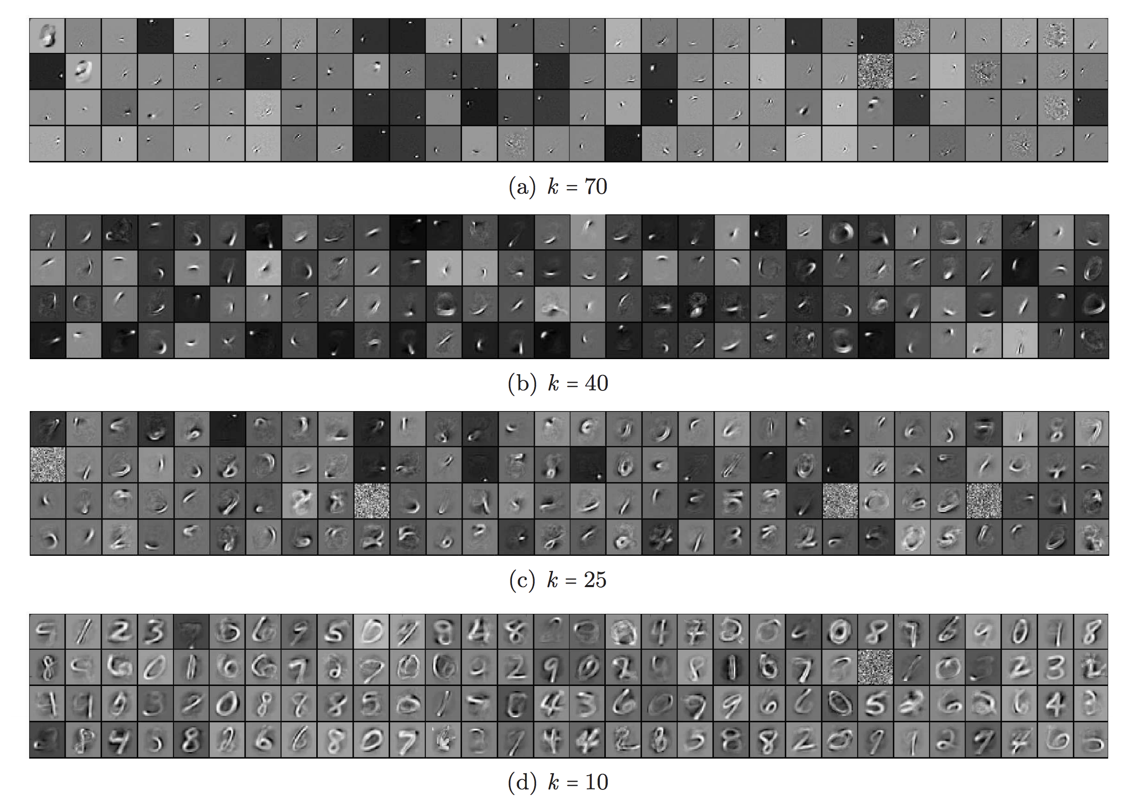
In the $k$-Sparse Autoencoder (Makhzani and Frey, 2013), sparsity is enforced by retaining only the top k highest activations in the bottleneck layer, which uses a linear activation function. First, run a feedforward pass through the encoder network to obtain the compressed code: $\mathbf{z} = g(\mathbf{x})$. Next, sort the values in the code vector $\mathbf{z}$. Keep only the k largest values and set the remaining neurons to 0. (This can also be implemented using a ReLU layer with an adjustable threshold.) This yields a sparsified code: $\mathbf{z}’ = \text{Sparsify}(\mathbf{z})$. Then compute the output and loss from the sparsified code, $L = |\mathbf{x} - f(\mathbf{z}’) |_2^2$. Finally, backpropagation is performed only through the top k activated hidden units.
Contractive Autoencoder
Like the sparse autoencoder, the Contractive Autoencoder (Rifai, et al, 2011) promotes robustness by encouraging the learned representation to remain within a contractive space.
It adds a term to the loss function that penalizes representations that are overly sensitive to the input, thereby improving robustness to small perturbations around training points. Sensitivity is quantified using the Frobenius norm of the Jacobian matrix of encoder activations with respect to the input:
where $h_j$ is one unit output in the compressed code $\mathbf{z} = f(x)$.
This penalty is the sum of squares of all partial derivatives of the learned encoding with respect to the input dimensions. The authors claimed that, empirically, this penalty was found to carve a representation aligned with a lower-dimensional non-linear manifold, while remaining more invariant along most directions orthogonal to that manifold.
VAE: Variational Autoencoder
The Variational Autoencoder (Kingma & Welling, 2014), abbreviated VAE, is in fact less similar to the autoencoder models above and is instead rooted in variational Bayesian methods and graphical models.
Rather than mapping an input to a fixed vector, we map it to a distribution. Denote this distribution as $p_\theta$, parameterized by $\theta$. The relationship between the data input $\mathbf{x}$ and the latent encoding vector $\mathbf{z}$ can be fully specified by:
- Prior $p_\theta(\mathbf{z})$
- Likelihood $p_\theta(\mathbf{x}\vert\mathbf{z})$
- Posterior $p_\theta(\mathbf{z}\vert\mathbf{x})$
Assume we know the true parameter $\theta^{*}$ for this distribution. To generate a sample that resembles a real data point $\mathbf{x}^{(i)}$, we proceed as follows:
- First, sample a $\mathbf{z}^{(i)}$ from a prior distribution $p_{\theta^*}(\mathbf{z})$.
- Then generate a value $\mathbf{x}^{(i)}$ from a conditional distribution $p_{\theta^*}(\mathbf{x} \vert \mathbf{z} = \mathbf{z}^{(i)})$.
The optimal parameter $\theta^{*}$ is the one that maximizes the probability of generating real data samples:
In practice, we often use log probabilities to convert the product on the RHS into a sum:
Now, rewrite the expression to make the data-generation process more explicit by incorporating the encoding vector:
Unfortunately, computing $p_\theta(\mathbf{x}^{(i)})$ this way is not easy, because it is very expensive to enumerate all possible values of $\mathbf{z}$ and sum them. To reduce the search space and enable faster inference, we introduce an approximation function that outputs a likely code given an input $\mathbf{x}$, namely $q_\phi(\mathbf{z}\vert\mathbf{x})$, parameterized by $\phi$.
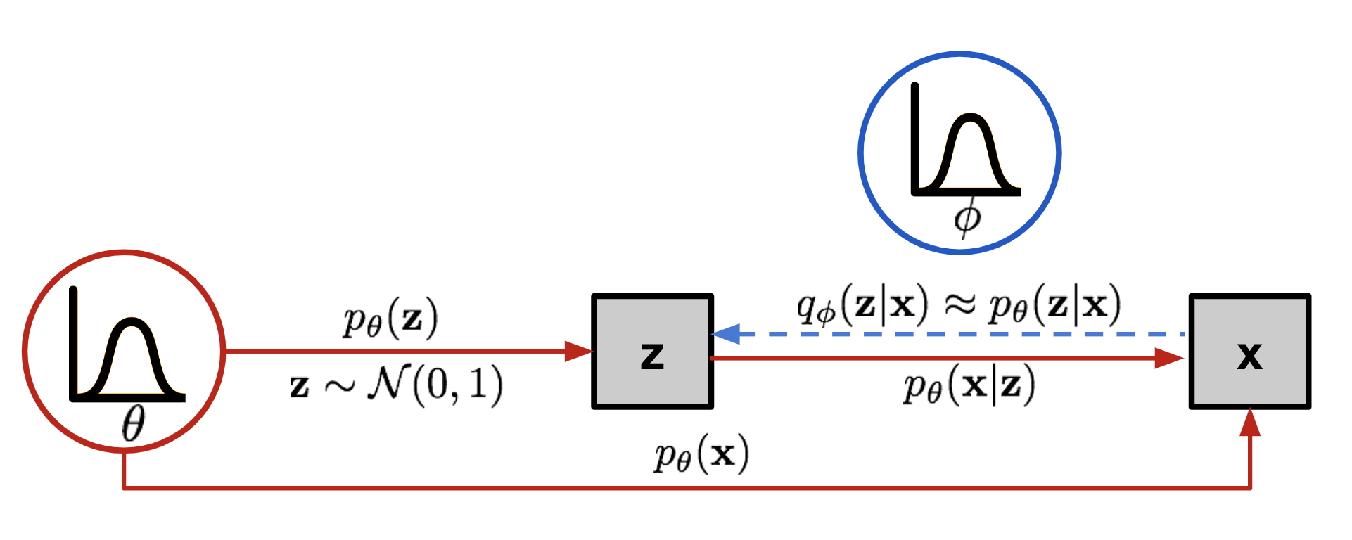
With this setup, the structure now closely resembles an autoencoder:
- The conditional probability $p_\theta(\mathbf{x} \vert \mathbf{z})$ defines a generative model, analogous to the decoder $f_\theta(\mathbf{x} \vert \mathbf{z})$ introduced earlier. $p_\theta(\mathbf{x} \vert \mathbf{z})$ is also referred to as the probabilistic decoder.
- The approximation function $q_\phi(\mathbf{z} \vert \mathbf{x})$ is the probabilistic encoder, serving a role similar to $g_\phi(\mathbf{z} \vert \mathbf{x})$ above.
Loss Function: ELBO
The estimated posterior $q_\phi(\mathbf{z}\vert\mathbf{x})$ should closely match the true posterior $p_\theta(\mathbf{z}\vert\mathbf{x})$. We can use Kullback-Leibler divergence to measure the distance between these two distributions. The KL divergence $D_\text{KL}(X|Y)$ quantifies how much information is lost when distribution Y is used to represent X.
In this setting, we aim to minimize $D_\text{KL}( q_\phi(\mathbf{z}\vert\mathbf{x}) | p_\theta(\mathbf{z}\vert\mathbf{x}) )$ with respect to $\phi$.
Why use $D_\text{KL}(q_\phi | p_\theta)$ (reversed KL) instead of $D_\text{KL}(p_\theta | q_\phi)$ (forward KL)? Eric Jang provides a strong explanation in his post on Bayesian Variational methods. As a brief recap:
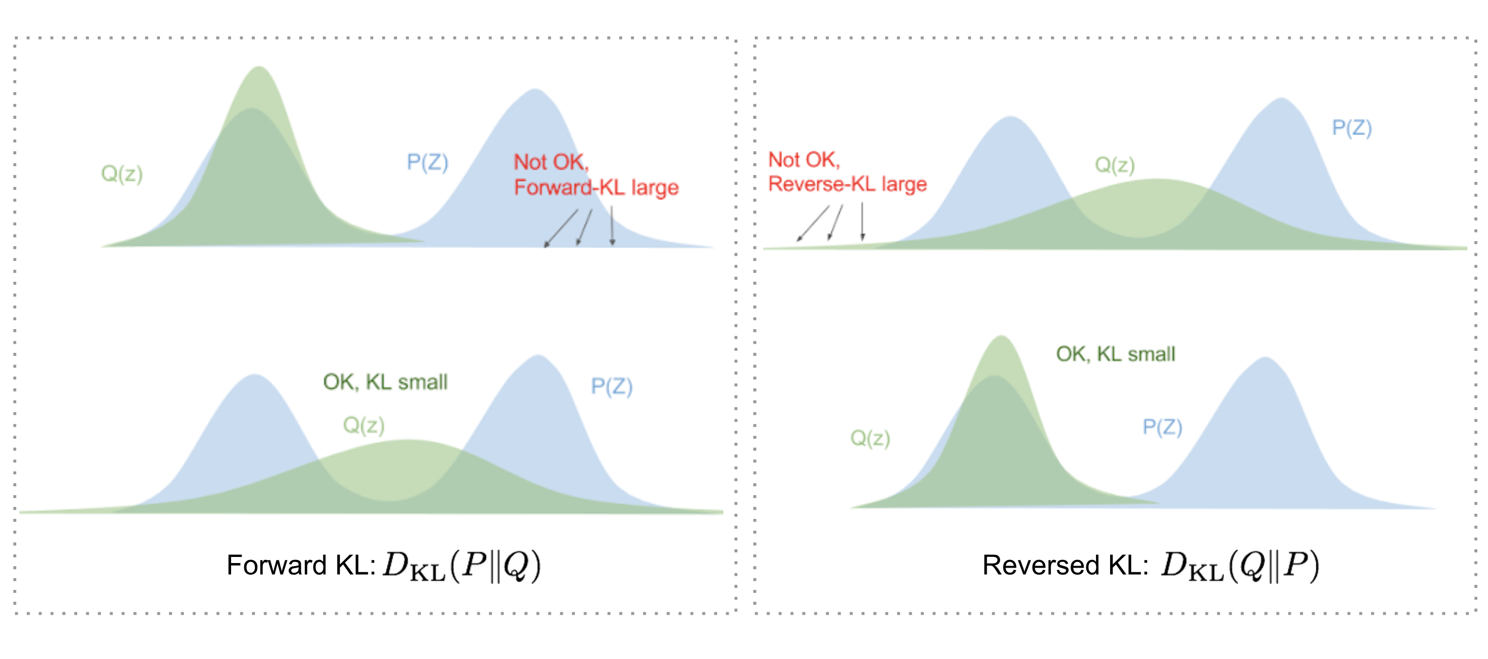
- Forward KL divergence: $D_\text{KL}(P|Q) = \mathbb{E}_{z\sim P(z)} \log\frac{P(z)}{Q(z)}$; we must ensure that Q(z)>0 wherever P(z)>0. The optimized variational distribution $q(z)$ must cover the entire $p(z)$.
- Reversed KL divergence: $D_\text{KL}(Q|P) = \mathbb{E}_{z\sim Q(z)} \log\frac{Q(z)}{P(z)}$; minimizing the reversed KL divergence squeezes the $Q(z)$ under $P(z)$.
Now expand the equation:
Therefore, we have:
After rearranging the left-hand and right-hand sides,
The LHS is exactly what we want to maximize when learning the true distributions: maximize the (log-)likelihood of generating real data (that is $\log p_\theta(\mathbf{x})$) and also minimize the gap between the true and estimated posterior distributions (the term $D_\text{KL}$ acts as a regularizer). Note that $p_\theta(\mathbf{x})$ is fixed with respect to $q_\phi$.
Taking the negative of the above yields the loss function:
In Variational Bayesian methods, this objective is known as the variational lower bound, or the evidence lower bound. The “lower bound” terminology comes from the fact that KL divergence is always non-negative, and therefore $-L_\text{VAE}$ is a lower bound of $\log p_\theta (\mathbf{x})$.
Consequently, minimizing the loss maximizes the lower bound on the probability of generating real data samples.
Reparameterization Trick
The expectation term in the loss requires generating samples from $\mathbf{z} \sim q_\phi(\mathbf{z}\vert\mathbf{x})$. Because sampling is stochastic, gradients cannot be backpropagated through it directly. To make training possible, the reparameterization trick is used: it is often possible to express the random variable $\mathbf{z}$ as a deterministic variable $\mathbf{z} = \mathcal{T}_\phi(\mathbf{x}, \boldsymbol{\epsilon})$, where $\boldsymbol{\epsilon}$ is an auxiliary independent random variable, and the transformation $\mathcal{T}_\phi$ parameterized by $\phi$ maps $\boldsymbol{\epsilon}$ to $\mathbf{z}$.
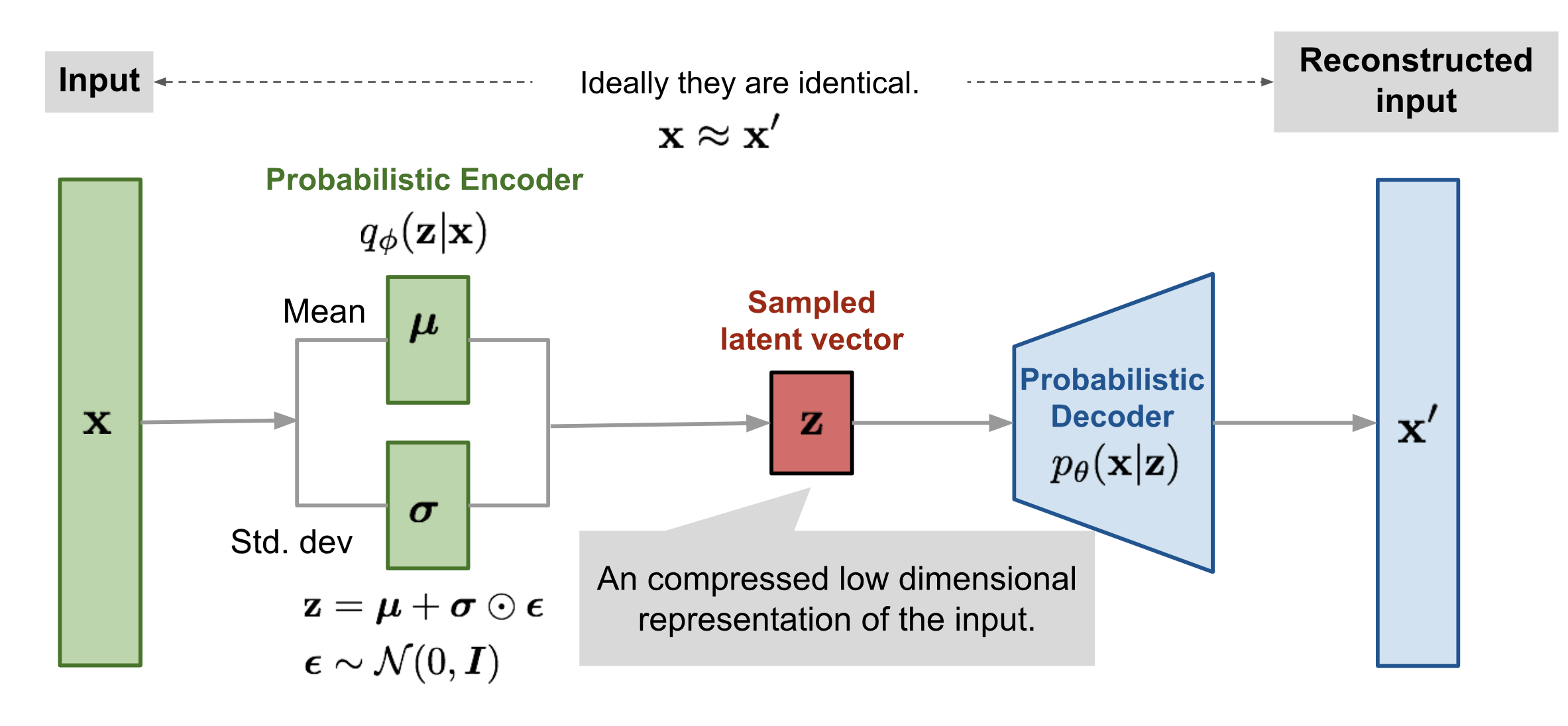
For example, a common choice for $q_\phi(\mathbf{z}\vert\mathbf{x})$ is a multivariate Gaussian with a diagonal covariance structure:
where $\odot$ denotes element-wise multiplication.
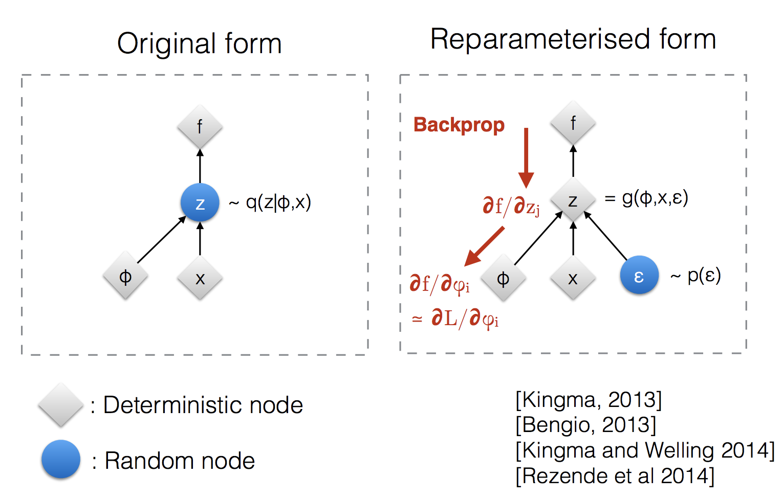
The reparameterization trick also applies to other types of distributions, not only Gaussian. In the multivariate Gaussian case, we make the model trainable by explicitly learning the mean and variance of the distribution, $\mu$ and $\sigma$, using the reparameterization trick, while the stochasticity remains in the random variable $\boldsymbol{\epsilon} \sim \mathcal{N}(0, \boldsymbol{I})$.
Beta-VAE
If each variable in the inferred latent representation $\mathbf{z}$ is sensitive to only one generative factor and is relatively invariant to other factors, then the representation is said to be disentangled, or factorized. A common benefit of disentangled representations is strong interpretability and easier generalization across a range of tasks.
For example, a model trained on photos of human faces might encode relatively independent factors (such as gender, skin color, hair color, hair length, emotion, and whether the person is wearing glasses) in separate dimensions. This type of disentangled representation is highly beneficial for facial image generation.
β-VAE (Higgins et al., 2017) modifies the Variational Autoencoder with a particular emphasis on discovering disentangled latent factors. Following the same motivation as in VAE, we aim to maximize the probability of generating real data while keeping the distance between the true and estimated posterior distributions small (for example, under a small constant $\delta$):
This can be rewritten as a Lagrangian, with a Lagrangian multiplier $\beta$ under the KKT condition. The optimization problem above, with a single inequality constraint, is equivalent to maximizing the following expression $\mathcal{F}(\theta, \phi, \beta)$:
The loss function of $\beta$-VAE is defined as:
Here, the Lagrangian multiplier $\beta$ is treated as a hyperparameter.
Because the negation of $L_\text{BETA}(\phi, \beta)$ forms the lower bound of the Lagrangian $\mathcal{F}(\theta, \phi, \beta)$, minimizing the loss is equivalent to maximizing the Lagrangian. Consequently, this objective aligns with our original optimization problem.
When $\beta=1$, the formulation reduces to the standard VAE. When $\beta > 1$, it enforces a stricter constraint on the latent bottleneck and therefore limits the representation capacity of $\mathbf{z}$. For generative factors that are conditionally independent, maintaining a disentangled structure is often the most efficient representation. As a result, a larger $\beta$ promotes a more efficient latent encoding and further encourages disentanglement. At the same time, increasing $\beta$ can introduce a trade-off between reconstruction fidelity and the degree of disentanglement.
Burgess, et al. (2017) examined disentanglement in $\beta$-VAE in depth, drawing inspiration from information bottleneck theory, and then proposed a modification to $\beta$-VAE to provide better control over encoding representation capacity.
VQ-VAE and VQ-VAE-2
The VQ-VAE (“Vector Quantised-Variational AutoEncoder”; van den Oord, et al. 2017) model uses the encoder to learn a discrete latent variable, motivated by the idea that discrete representations may better match domains such as language, speech, and reasoning.
Vector quantisation (VQ) maps $K$-dimensional vectors into a finite collection of “code” vectors. This procedure is closely related to the KNN algorithm. The optimal centroid code vector for a given sample is the one that minimizes Euclidean distance.
Let $\mathbf{e} \in \mathbb{R}^{K \times D}, i=1, \dots, K$ denote the latent embedding space (also called the “codebook”) in VQ-VAE, where $K$ is the number of latent variable categories and $D$ is the embedding dimensionality. A single embedding vector is $\mathbf{e}_i \in \mathbb{R}^{D}, i=1, \dots, K$.
The encoder output $E(\mathbf{x}) = \mathbf{z}_e$ is passed through a nearest-neighbor lookup to select one of the $K$ embedding vectors. The selected code vector is then provided to the decoder $D(.)$:
Note that discrete latent variables may take different shapes depending on the application, for example, 1D for speech, 2D for images, and 3D for video.
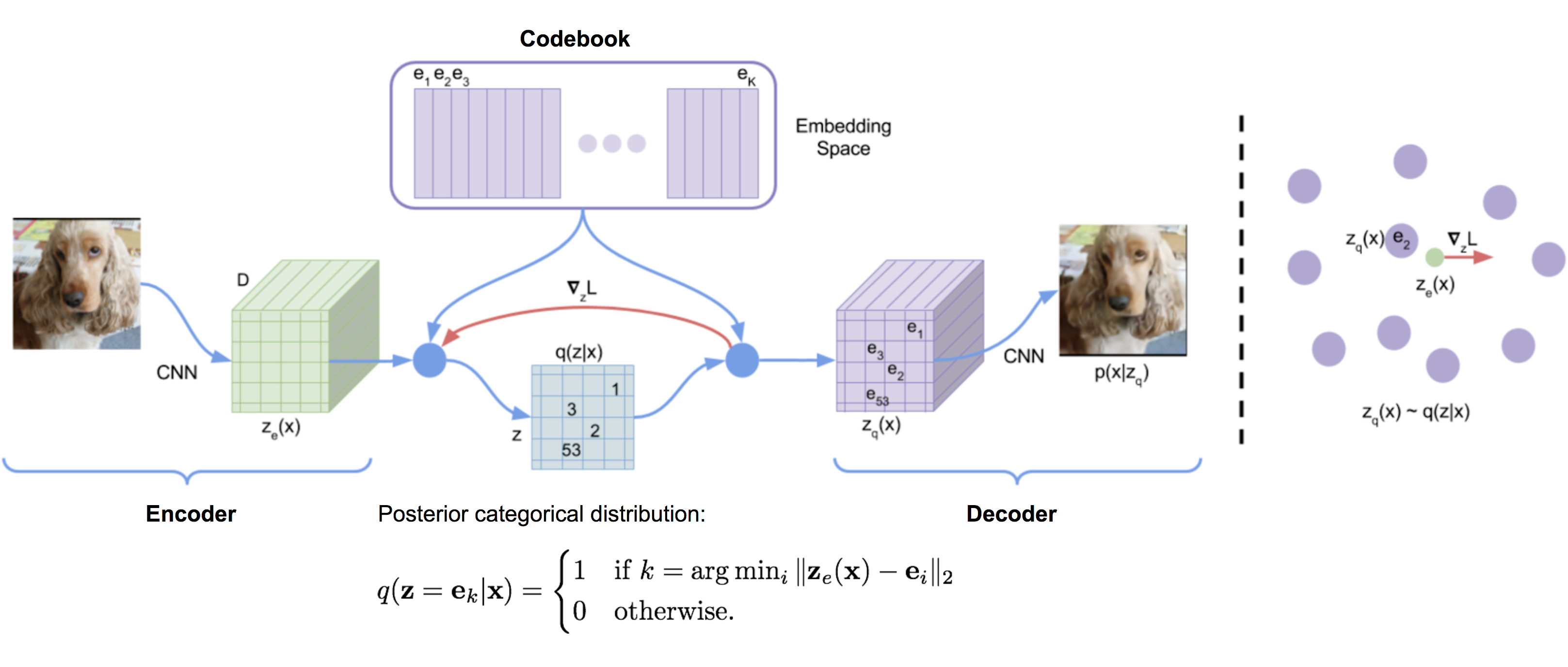
Because argmin() is non-differentiable over a discrete space, the gradients $\nabla_z L$ from the decoder input $\mathbf{z}_q$ are copied back to the encoder output $\mathbf{z}_e$. In addition to the reconstruction loss, VQ-VAE also optimizes the following terms:
- VQ loss: The L2 error between the embedding space and the encoder outputs.
- Commitment loss: A term that encourages the encoder output to remain close to the embedding space and prevents it from switching too frequently between code vectors.
where $\text{sg}[.]$ is the stop_gradient operator.
The embedding vectors in the codebook are updated using EMA (exponential moving average). For a code vector $\mathbf{e}_i$, suppose there are $n_i$ encoder output vectors, $\{\mathbf{z}_{i,j}\}_{j=1}^{n_i}$, that are quantized to $\mathbf{e}_i$:
where $(t)$ denotes the batch sequence in time. $N_i$ and $\mathbf{m}_i$ represent the accumulated vector count and volume, respectively.
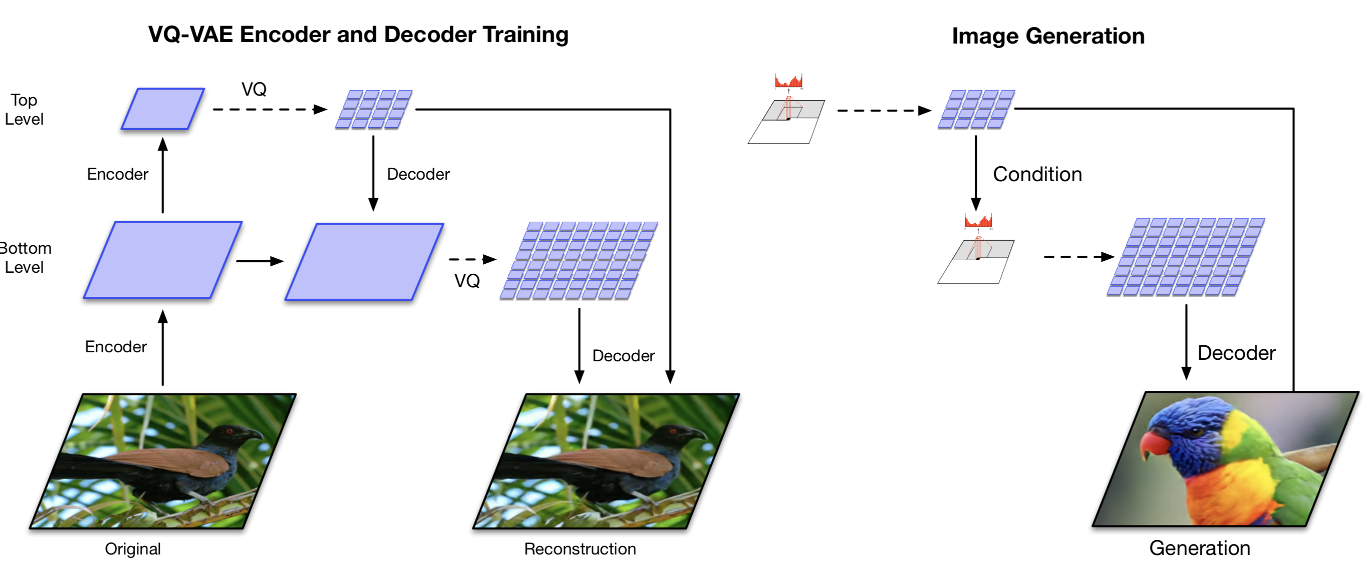
VQ-VAE-2 (Ali Razavi, et al. 2019) extends VQ-VAE into a two-level hierarchical architecture and combines it with a self-attention autoregressive model.
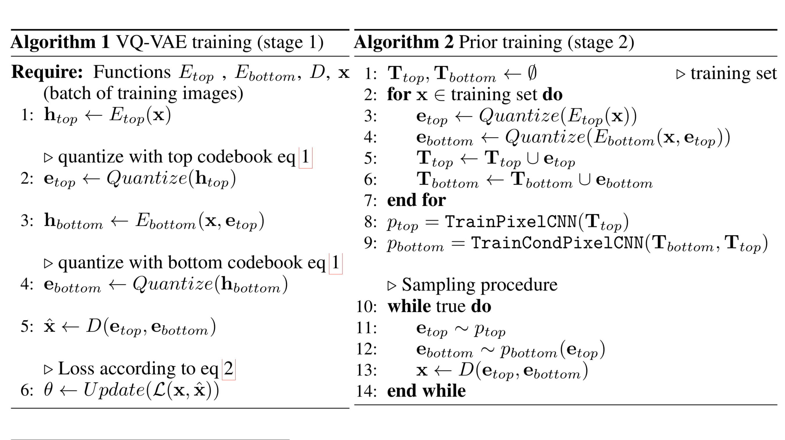
- Stage 1: Train a hierarchical VQ-VAE. The hierarchical latent-variable design is intended to separate local patterns (for example, texture) from global information (for example, object shapes). Training for the larger bottom-level codebook is also conditioned on the smaller top-level code, so it does not need to learn everything from scratch.
- Stage 2: Learn a prior over the latent discrete codebook, enabling sampling and image generation. This approach ensures that the decoder receives input vectors drawn from a distribution similar to the one observed during training. A strong autoregressive model, augmented with multi-headed self-attention layers, is used to model the prior distribution (such as PixelSNAIL; Chen et al 2017).
Given that VQ-VAE-2 relies on discrete latent variables arranged in a straightforward hierarchical structure, the quality of its generated images is quite remarkable.
TD-VAE
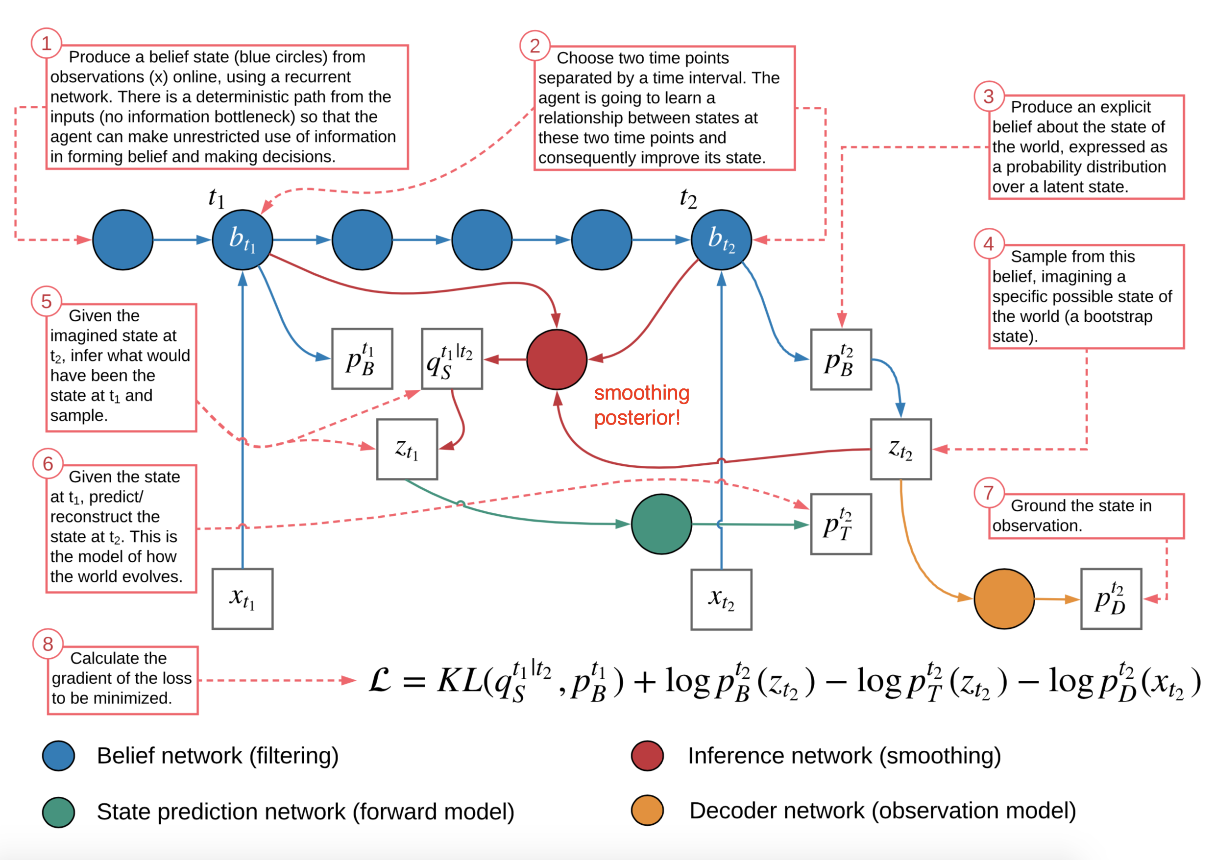
TD-VAE (“Temporal Difference VAE”; Gregor et al., 2019) is designed for sequential data. It is built on three core ideas, outlined below.
1. State-Space Models
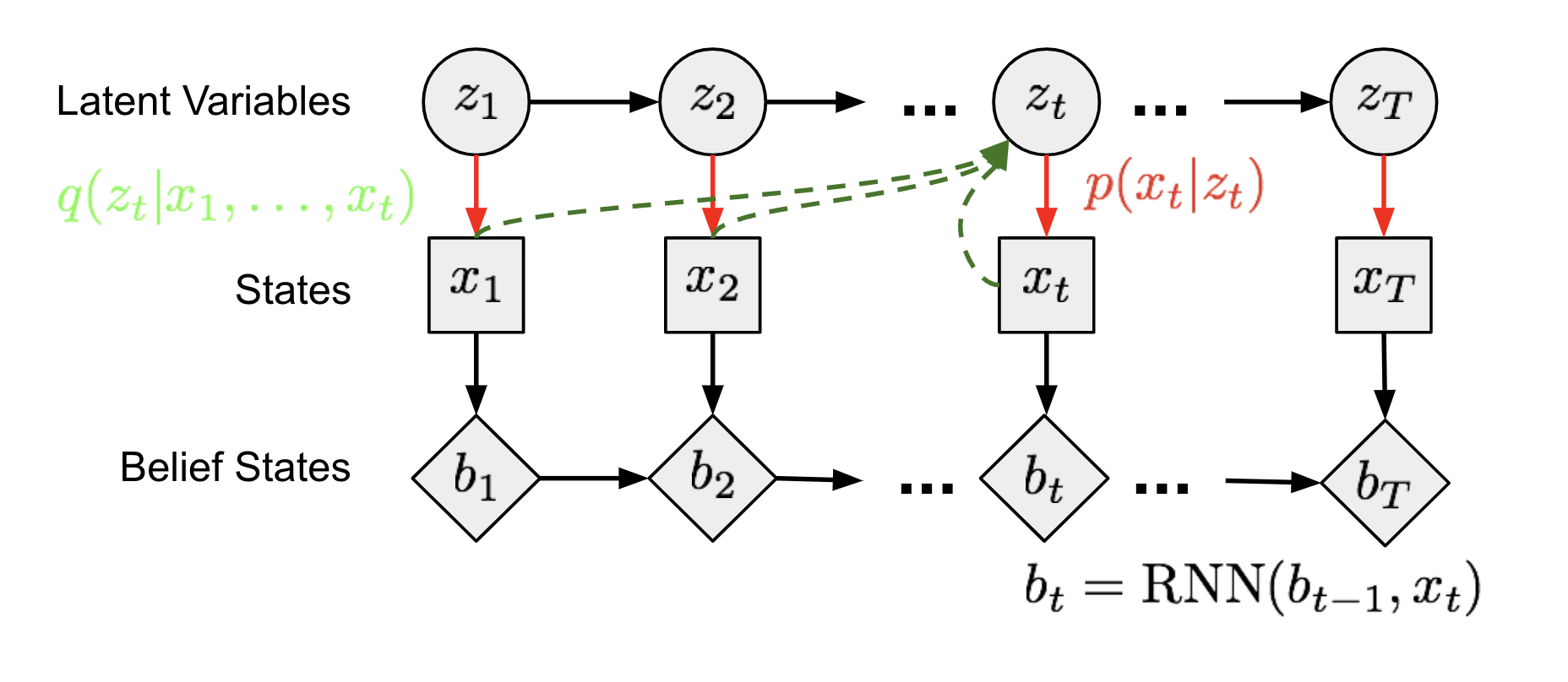
In (latent) state-space models, a sequence of unobserved hidden states $\mathbf{z} = (z_1, \dots, z_T)$ determines the observation states $\mathbf{x} = (x_1, \dots, x_T)$. Each time step in the Markov chain model in Fig. 13 can be trained in a manner similar to Fig. 6, where the intractable posterior $p(z \vert x)$ is approximated by a function $q(z \vert x)$.
2. Belief State
An agent should learn to encode all past states in order to reason about the future. This representation is referred to as the belief state, $b_t = belief(x_1, \dots, x_t) = belief(b_{t-1}, x_t)$. Under this definition, the distribution of future states conditioned on the past can be expressed as $p(x_{t+1}, \dots, x_T \vert x_1, \dots, x_t) \approx p(x_{t+1}, \dots, x_T \vert b_t)$. TD-VAE uses the hidden states in a recurrent policy as the agent’s belief state. Therefore, we obtain $b_t = \text{RNN}(b_{t-1}, x_t)$.
3. Jumpy Prediction
In addition, an agent is expected to imagine distant futures using all information accumulated so far. This motivates the ability to make jumpy predictions, meaning predictions of states several steps into the future.
Recall what we have learned from the variance lower bound above:
Now, model the distribution of the state $x_t$ as a probability function conditioned on all past states $x_{
Continue by expanding the equation:
Note the following:
- The red terms can be ignored under the Markov assumptions.
- The blue term is expanded according to the Markov assumptions.
- The green term is expanded to include a one-step prediction back into the past, serving as a smoothing distribution.
More precisely, there are four categories of distributions to learn:
- $p_D(.)$ is the decoder distribution:
- $p(x_t \mid z_t)$ is the encoder under the standard definition;
- $p(x_t \mid z_t) \to p_D(x_t \mid z_t)$;
- $p_T(.)$ is the transition distribution:
- $p(z_t \mid z_{t-1})$ captures the sequential dependency between latent variables;
- $p(z_t \mid z_{t-1}) \to p_T(z_t \mid z_{t-1})$;
- $p_B(.)$ is the belief distribution:
- Both $p(z_{t-1} \mid x_{
- $p(z_{t-1} \mid x_{
- $q(z_{t} \mid x_{\leq t}) \to p_B(z_t \mid b_t)$;
- $p_S(.)$ is the smoothing distribution:
- The back-to-past smoothing term $q(z_{t-1} \mid z_t, x_{\leq t})$ can be rewritten to depend on belief states as well;
- $q(z_{t-1} \mid z_t, x_{\leq t}) \to p_S(z_{t-1} \mid z_t, b_{t-1}, b_t)$;
To incorporate jumpy prediction, the sequential ELBO must operate not only on $t, t+1$, but also across two distant timestamps $t_1 < t_2$. The following is the final TD-VAE objective function to maximize:
Cited as:
@article{weng2018VAE,
  title   = "From Autoencoder to Beta-VAE",
  author  = "Weng, Lilian",
  journal = "lilianweng.github.io",
  year    = "2018",
  url     = "https://lilianweng.github.io/posts/2018-08-12-vae/"
}
References
[1] Geoffrey E. Hinton, and Ruslan R. Salakhutdinov. “Reducing the dimensionality of data with neural networks.” Science 313.5786 (2006): 504-507.
[2] Pascal Vincent, et al. “Extracting and composing robust features with denoising autoencoders.” ICML, 2008.
[3] Pascal Vincent, et al. “Stacked denoising autoencoders: Learning useful representations in a deep network with a local denoising criterion.”. Journal of machine learning research 11.Dec (2010): 3371-3408.
[4] Geoffrey E. Hinton, Nitish Srivastava, Alex Krizhevsky, Ilya Sutskever, and Ruslan R. Salakhutdinov. “Improving neural networks by preventing co-adaptation of feature detectors.” arXiv preprint arXiv:1207.0580 (2012).
[5] Sparse Autoencoder by Andrew Ng.
[6] Alireza Makhzani, Brendan Frey (2013). “k-sparse autoencoder”. ICLR 2014.
[7] Salah Rifai, et al. “Contractive auto-encoders: Explicit invariance during feature extraction.” ICML, 2011.
[8] Diederik P. Kingma, and Max Welling. “Auto-encoding variational bayes.” ICLR 2014.
[9] Tutorial - What is a variational autoencoder? on jaan.io
[10] Youtube tutorial: Variational Autoencoders by Arxiv Insights
[11] “A Beginner’s Guide to Variational Methods: Mean-Field Approximation” by Eric Jang.
[12] Carl Doersch. “Tutorial on variational autoencoders.” arXiv:1606.05908, 2016.
[13] Irina Higgins, et al. "$\beta$-VAE: Learning basic visual concepts with a constrained variational framework." ICLR 2017.
[14] Christopher P. Burgess, et al. “Understanding disentangling in beta-VAE.” NIPS 2017.
[15] Aaron van den Oord, et al. “Neural Discrete Representation Learning” NIPS 2017.
[16] Ali Razavi, et al. “Generating Diverse High-Fidelity Images with VQ-VAE-2”. arXiv preprint arXiv:1906.00446 (2019).
[17] Xi Chen, et al. “PixelSNAIL: An Improved Autoregressive Generative Model.” arXiv preprint arXiv:1712.09763 (2017).
[18] Karol Gregor, et al. “Temporal Difference Variational Auto-Encoder.” ICLR 2019.