Meta-Learning: Learning to Learn Fast
[Updated on 2019-10-01: with thanks to Tianhao, this post is now available in a Chinese translation!]
· 30 min read · Curated and presented by Arthur Sedek
[Updated on 2019-10-01: thanks to Tianhao, we have this post translated in Chinese!]
In many machine learning settings, strong performance depends on training with a large number of samples. Humans, by contrast, often learn new concepts and skills far more quickly and efficiently. Children who have seen cats and birds only a few times can readily distinguish between them. Likewise, someone who already knows how to ride a bicycle can often figure out how to ride a motorcycle rapidly, with little or even no demonstration. Can we design machine learning models with comparable properties, namely, the ability to learn new concepts and skills quickly from only a few examples? That is the central problem that meta-learning is intended to address.
A capable meta-learning model should adapt or generalize effectively to new tasks and environments that were not encountered during training. This adaptation, essentially a small learning session, occurs at test time, but under limited exposure to new task configurations. After adaptation, the model should be able to complete the new tasks. This is why meta-learning is also known as learning to learn.
The tasks can come from any well-defined family of machine learning problems, including supervised learning, reinforcement learning, and others. For example, the following are concrete meta-learning tasks:
- A classifier trained on non-cat images can determine whether a given image contains a cat after seeing only a handful of cat pictures.
- A game bot can quickly learn to master a new game.
- A small robot can complete a desired task on an uphill surface at test time even through it was trained only in a flat-surface environment.
Define the Meta-Learning Problem
In this post, we focus on the case where each target task is a supervised learning problem, such as image classification. There is extensive and interesting literature on meta-learning in reinforcement learning settings (also known as “Meta Reinforcement Learning”), but we do not cover that topic here.
A Simple View
A meta-learning model should be trained across a wide variety of learning tasks and optimized to perform well over a distribution of tasks, including tasks that may be unseen. Each task is associated with a dataset $\mathcal{D}$, which includes both feature vectors and ground-truth labels. The optimal model parameters are:
This formulation closely resembles standard learning, except that one dataset is treated as one data sample.
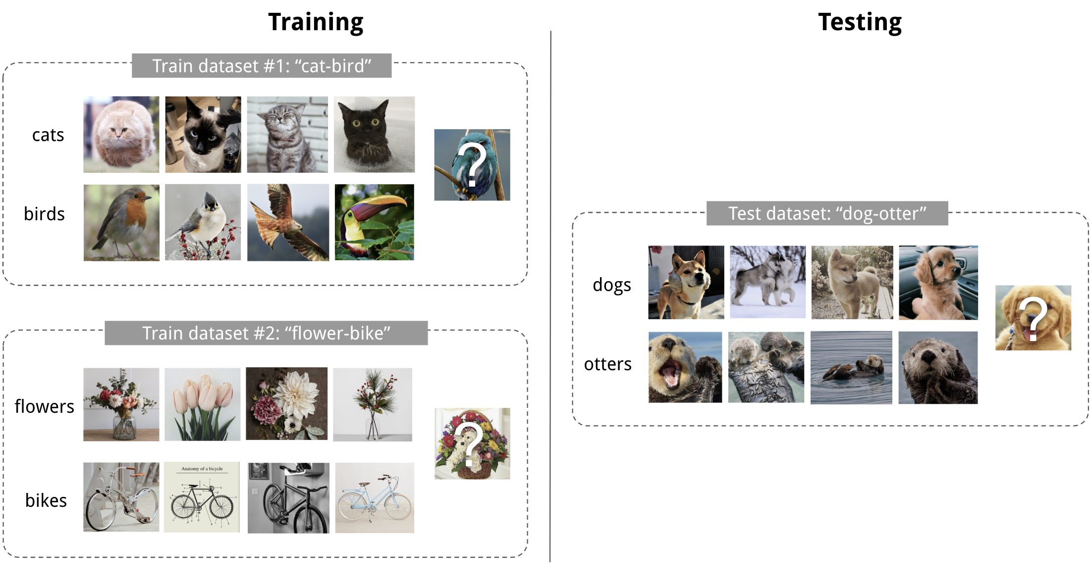
Few-shot classification is a common instantiation of meta-learning in supervised learning. The dataset $\mathcal{D}$ is often divided into two parts: a support set $S$ for learning and a prediction set $B$ for training or testing, $\mathcal{D}=\langle S, B\rangle$. A frequent setup is a K-shot N-class classification task, where the support set contains K labeled examples for each of N classes.
Training in the Same Way as Testing
A dataset $\mathcal{D}$ consists of feature vector and label pairs, $\mathcal{D} = \{(\mathbf{x}_i, y_i)\}$, where each label belongs to a known label set $\mathcal{L}^\text{label}$. Suppose our classifier $f_\theta$, with parameters $\theta$, outputs the probability that a data point belongs to class $y$ given feature vector $\mathbf{x}$, $P_\theta(y\vert\mathbf{x})$.
The optimal parameters maximize the probability of the true labels across multiple training batches $B \subset \mathcal{D}$:
In few-shot classification, the objective is to reduce prediction error on samples with unknown labels, given only a small support set for “fast learning” (analogous to how “fine-tuning” works). To ensure that training mirrors inference behavior, we would like to “fake” datasets by restricting each episode to a subset of labels, thereby preventing the model from being exposed to all labels at once. We then adjust the optimization procedure accordingly to encourage fast adaptation:
- Sample a subset of labels, $L\subset\mathcal{L}^\text{label}$.
- Sample a support set $S^L \subset \mathcal{D}$ and a training batch $B^L \subset \mathcal{D}$. Both contain only data points whose labels belong to the sampled label set $L$, $y \in L, \forall (x, y) \in S^L, B^L$.
- The support set is included as part of the model input.
- In the final optimization step, use the mini-batch $B^L$ to compute the loss and update model parameters via backpropagation, in the same manner as in supervised learning.
You can treat each sampled dataset pair $(S^L, B^L)$ as a single data point. The model is trained to generalize to other datasets. Symbols shown in red are introduced for meta-learning in addition to the supervised learning objective.
This idea is related to using a pre-trained model for image classification (ImageNet) or language modeling (large text corpora) when only a limited amount of task-specific data is available. Meta-learning extends the idea further: instead of fine-tuning for a single downstream task, it optimizes the model to perform well across many tasks, if not all.
Learner and Meta-Learner
Another common perspective on meta-learning decomposes the update procedure into two stages:
- A classifier $f_\theta$ serves as the “learner” model, trained to solve a particular task.
- At the same time, an optimizer $g_\phi$ learns how to update the learner’s parameters using the support set $S$, $\theta’ = g_\phi(\theta, S)$.
In the final optimization step, both $\theta$ and $\phi$ must be updated to maximize:
Common Approaches
Three major families of meta-learning methods are commonly discussed: metric-based, model-based, and optimization-based. Oriol Vinyals provides a helpful summary in his talk at meta-learning symposium @ NIPS 2018:
| ,,,,- | ,,,,- | ,,,,- | ,,,,- |
| Model-based | Metric-based | Optimization-based | |
|---|---|---|---|
| Key idea | RNN; memory | Metric learning | Gradient descent |
| How $P_\theta(y \vert \mathbf{x})$ is modeled? | $f_\theta(\mathbf{x}, S)$ | $\sum_{(\mathbf{x}_i, y_i) \in S} k_\theta(\mathbf{x}, \mathbf{x}_i)y_i$ (*) | $P_{g_\phi(\theta, S^L)}(y \vert \mathbf{x})$ |
(*) $k_\theta$ is a kernel function measuring the similarity between $\mathbf{x}_i$ and $\mathbf{x}$.
Next, we review classic models within each approach.
Metric-Based
The central concept in metric-based meta-learning is closely related to nearest-neighbors methods (for example, k-NN classificer and k-means clustering) and kernel density estimation. The predicted probability over a set of known labels $y$ is computed as a weighted sum over the labels of support set samples. The weights are produced by a kernel function $k_\theta$ that measures the similarity between two data samples.
Learning a strong kernel is essential to the effectiveness of metric-based meta-learning. Metric learning is closely aligned with this goal, as it seeks to learn a metric or distance function over objects. What constitutes a good metric depends on the problem: it should reflect relationships among inputs in the task space and support effective problem solving.
All models introduced below explicitly learn embedding vectors for inputs and use those embeddings to construct appropriate kernel functions.
Convolutional Siamese Neural Network
The Siamese Neural Network consists of two twin networks whose outputs are trained jointly, using a function designed to learn the relationship between pairs of input samples. The two networks are identical and share the same weights and parameters. Put differently, both branches implement the same embedding network, which learns an effective representation for capturing relationships between pairs of data points.
Koch, Zemel & Salakhutdinov (2015) proposed applying a siamese neural network to one-shot image classification. The method first trains the siamese network on a verification task that determines whether two input images belong to the same class. The network outputs the probability that the two images come from the same class. At test time, the siamese network evaluates all pairs formed by the test image and each image in the support set. The predicted class is taken to be the class of the support image that yields the highest probability.
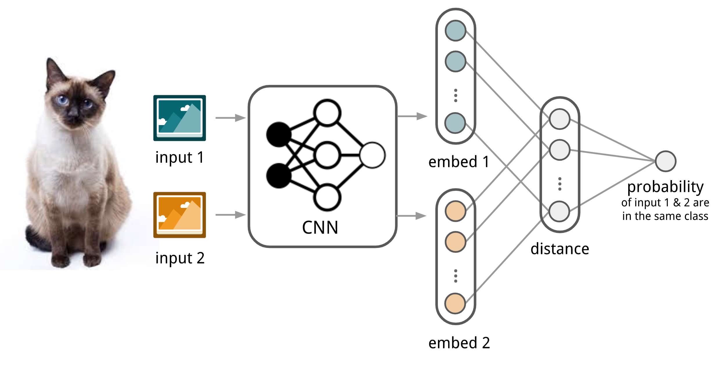
- First, the convolutional siamese network learns to encode two images into feature vectors via an embedding function $f_\theta$, which contains several convolutional layers.
- The L1-distance between two embeddings is $\vert f_\theta(\mathbf{x}_i) - f_\theta(\mathbf{x}_j) \vert$.
- This distance is mapped to a probability $p$ using a linear feedforward layer followed by a sigmoid. The resulting value represents the probability that the two images are drawn from the same class.
- Because the label is binary, the loss is naturally cross-entropy.
Images in the training batch $B$ may be augmented using distortions. Naturally, the L1 distance can be replaced by other distance metrics (L2, cosine, and so on). The key requirement is that the metric be differentiable; under that condition, the remaining components operate in the same way.
Given a support set $S$ and a test image $\mathbf{x}$, the final predicted class is:
where $c(\mathbf{x})$ denotes the class label of an image $\mathbf{x}$, and $\hat{c}(.)$ is the predicted label.
This approach assumes that the learned embedding generalizes well enough to measure distances between images from previously unseen categories. This is the same premise underlying transfer learning through the use of a pre-trained model. For example, convolutional features learned from a model pre-trained on ImageNet are expected to benefit other vision tasks. However, the usefulness of a pre-trained model typically declines as the new task diverges from the original training task.
Matching Networks
Matching Networks (Vinyals et al., 2016) aim to learn a classifier $c_S$ that can operate for any given (small) support set $S=\{x_i, y_i\}_{i=1}^k$ (k-shot classification). The classifier defines a probability distribution over output labels $y$ given a test example $\mathbf{x}$. As in other metric-based methods, the classifier output is expressed as a sum of labels for support samples, weighted by an attention kernel $a(\mathbf{x}, \mathbf{x}_i)$, which should be proportional to the similarity between $\mathbf{x}$ and $\mathbf{x}_i$.
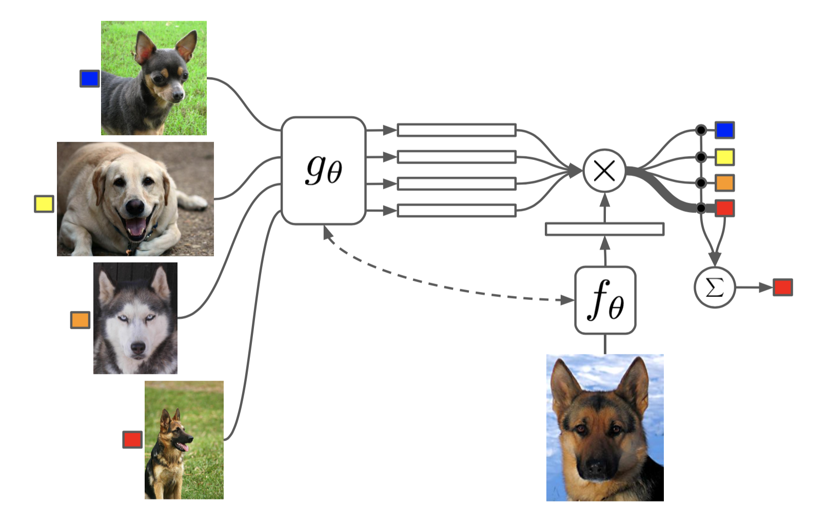
The attention kernel is defined using two embedding functions, $f$ and $g$, which encode the test sample and the support samples, respectively. The attention weight between two data points is computed as the cosine similarity, $\text{cosine}(.)$, between their embeddings and then normalized with a softmax:
Simple Embedding
In the simple configuration, the embedding function is a neural network that takes a single sample as input. Potentially we can set $f=g$.
Full Context Embeddings
Embedding vectors are critical for constructing an effective classifier. Using only a single data point as input may be insufficient to characterize the overall feature space. For this reason, Matching Networks further propose enhancing the embedding functions by providing the entire support set $S$ (in addition to the original input), allowing the embedding to be adjusted according to relationships among support samples.
-
$g_\theta(\mathbf{x}_i, S)$ uses a bidirectional LSTM to encode $\mathbf{x}_i$ in the context of the complete support set $S$.
-
$f_\theta(\mathbf{x}, S)$ encodes the test sample $\mathbf{x}$ visa an LSTM with read attention over the support set $S$.
- First, the test sample is passed through a simple neural network (for example, a CNN) to extract basic features, $f’(\mathbf{x})$.
- Next, an LSTM is trained where a read-attention vector over the support set is included as part of the hidden state:
$ \begin{aligned} \hat{\mathbf{h}}_t, \mathbf{c}_t &= \text{LSTM}(f'(\mathbf{x}), [\mathbf{h}_{t-1}, \mathbf{r}_{t-1}], \mathbf{c}_{t-1}) \\ \mathbf{h}_t &= \hat{\mathbf{h}}_t + f'(\mathbf{x}) \\ \mathbf{r}_{t-1} &= \sum_{i=1}^k a(\mathbf{h}_{t-1}, g(\mathbf{x}_i)) g(\mathbf{x}_i) \\ a(\mathbf{h}_{t-1}, g(\mathbf{x}_i)) &= \text{softmax}(\mathbf{h}_{t-1}^\top g(\mathbf{x}_i)) = \frac{\exp(\mathbf{h}_{t-1}^\top g(\mathbf{x}_i))}{\sum_{j=1}^k \exp(\mathbf{h}_{t-1}^\top g(\mathbf{x}_j))} \end{aligned} $- Finally, $f(\mathbf{x}, S)=\mathbf{h}_K$ after performing K “read” steps.
This embedding approach is referred to as “Full Contextual Embeddings (FCE)”. Notably, it improves performance on a challenging task (few-shot classification on mini ImageNet), but yields no measurable change on an easier task (Omniglot).
The training procedure for Matching Networks is explicitly designed to match test-time inference; see the details in the earlier section. It is worth noting that the Matching Networks paper sharpened the principle that training and testing conditions should align.
Relation Network
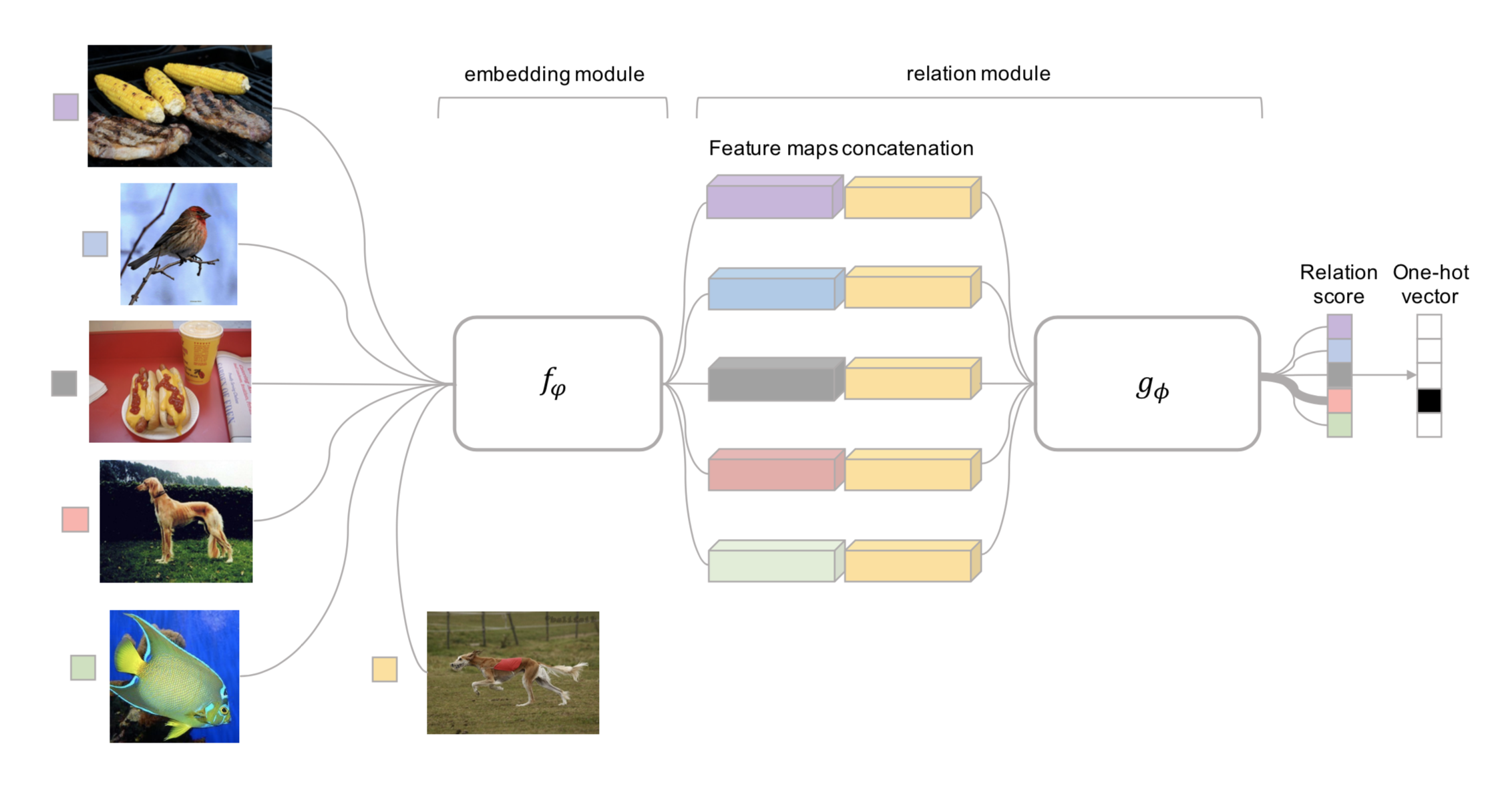
Relation Network (RN) (Sung et al., 2018) is similar to siamese network, but differs in several key respects:
- Relationships are not computed via a simple L1 distance in feature space. Instead, they are predicted by a CNN classifier $g_\phi$. The relation score for an input pair, $\mathbf{x}_i$ and $\mathbf{x}_j$, is $r_{ij} = g_\phi([\mathbf{x}_i, \mathbf{x}_j])$, where $[.,.]$ denotes concatenation.
- The objective uses MSE loss rather than cross-entropy, because RN is framed as predicting relation scores (a regression-like target) rather than performing binary classification, $\mathcal{L}(B) = \sum_{(\mathbf{x}_i, \mathbf{x}_j, y_i, y_j)\in B} (r_{ij} - \mathbf{1}_{y_i=y_j})^2$.
(Note: There is another Relation Network for relational reasoning, proposed by DeepMind. Don’t get confused.)
Prototypical Networks
Prototypical Networks (Snell, Swersky & Zemel, 2017) use an embedding function $f_\theta$ to map each input to a $M$-dimensional feature vector. For each class $c \in \mathcal{C}$, a prototype vector is defined as the mean of the embedded support samples in that class.
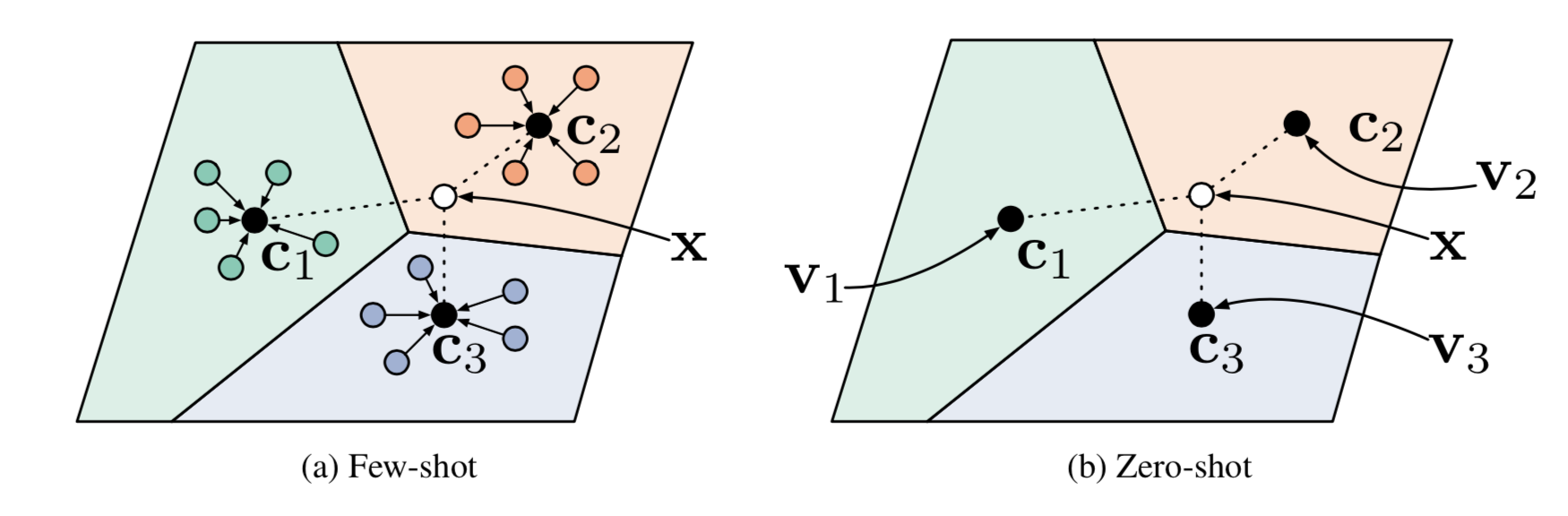
For a test input $\mathbf{x}$, the class distribution is computed as a softmax over the inverse distances between the test embedding and the prototype vectors.
Here, $d_\varphi$ may be any distance function, provided that $\varphi$ is differentiable. In the paper, the squared Euclidean distance is used.
The loss is the negative log-likelihood: $\mathcal{L}(\theta) = -\log P_\theta(y=c\vert\mathbf{x})$.
Model-Based
Model-based meta-learning methods do not assume any fixed form for $P_\theta(y\vert\mathbf{x})$. Instead, they rely on architectures designed specifically for fast learning, meaning models that can update their parameters rapidly within a small number of training steps. Such rapid updates may be enabled by the model’s internal structure or directed by a separate meta-learner.
Memory-Augmented Neural Networks
A family of model architectures introduces external memory to support the learning process in neural networks, including Neural Turing Machines and Memory Networks. With an explicit storage buffer, the network can incorporate new information quickly while reducing future forgetting. Models of this type are known as MANN, short for “Memory-Augmented Neural Network”. Note that recurrent neural networks with only internal memory (such as a vanilla RNN or an LSTM) are not MANNs.
Because MANN is expected to encode new information quickly and thereby adapt to new tasks after only a few samples, it is a natural fit for meta-learning. Using the Neural Turing Machine (NTM) as the base model, Santoro et al. (2016) introduced modifications to both the training setup and the memory retrieval mechanisms (also called “addressing mechanisms”, which determine how attention weights are assigned to memory vectors). If you are not already familiar with this topic, please review the NTM section in my other post before continuing.
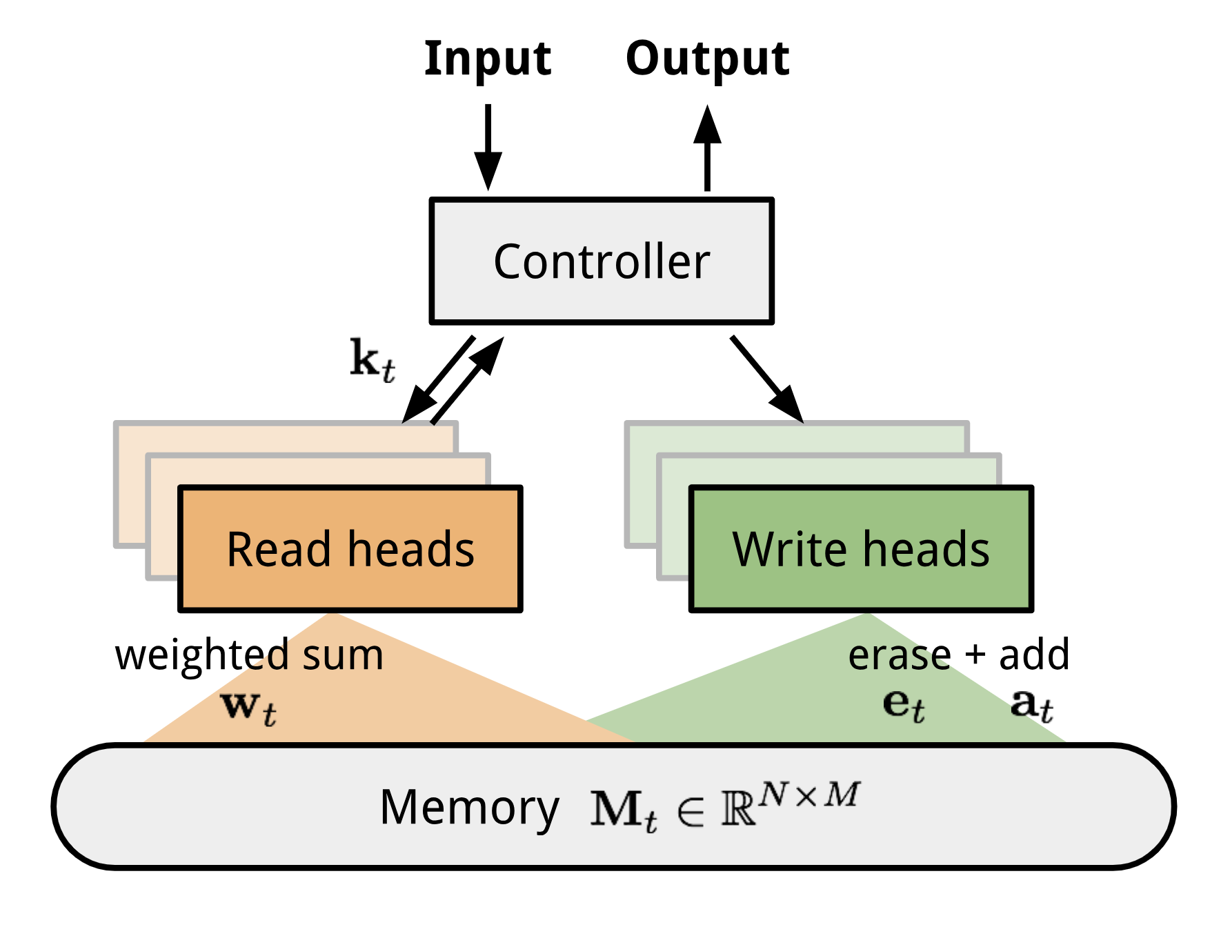
As a brief recap, NTM combines a controller neural network with external memory storage. The controller learns to read from and write to memory rows using soft attention, while the memory functions as a knowledge repository. Attention weights are produced by an addressing mechanism that combines content-based and location-based addressing.
MANN for Meta-Learning
To apply MANN to meta-learning, we must train it so that the memory can quickly encode and capture information about new tasks while ensuring that stored representations remain easy and stable to access.
The training procedure described in Santoro et al., 2016 is structured in a distinctive way so that memory is compelled to retain information longer, until the corresponding labels are presented at a later time. In each training episode, the true label $y_t$ is provided with a one step offset, $(\mathbf{x}_{t+1}, y_t)$: it is the correct label for the input at the previous time step t, but it is presented as part of the input at time step t+1.
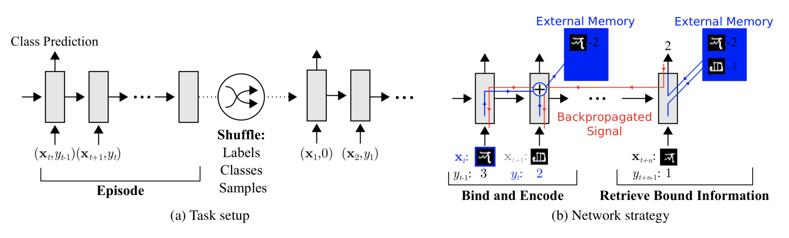
This setup encourages MANN to memorize information from a new dataset. The memory must retain the current input until the label becomes available later, and then retrieve the earlier information to produce the appropriate prediction.
Next, we examine how memory is updated to enable efficient storage and retrieval.
Addressing Mechanism for Meta-Learning
In addition to the training procedure, a new addressing mechanism that is purely content-based is used to make the model better suited to meta-learning.
» How to read from memory?
Read attention is constructed solely from content similarity.
First, at time step t the controller produces a key vector $\mathbf{k}_t$ as a function of the input $\mathbf{x}$. As in NTM, a read weighting vector $\mathbf{w}_t^r$ with N elements is computed as the cosine similarity between the key and each memory row, then normalized by a softmax. The read vector $\mathbf{r}_t$ is the weighted sum of memory records under these weightings:
where $M_t$ is the memory matrix at time t, and $M_t(i)$ denotes the i-th row of this matrix.
» How to write into memory?
The mechanism used to write newly received information into memory closely resembles the cache replacement policy. The Least Recently Used Access (LRUA) writer is introduced for MANN to improve performance specifically in meta-learning scenarios. An LRUA write head prefers to write new content either to the least used memory location or to the most recently used memory location.
- Infrequently accessed locations: this helps preserve information that is used often (see LFU);
- The most recently used location: the rationale is that once a piece of information has been retrieved, it is unlikely to be needed again for some time (see MRU).
A wide range of cache replacement algorithms exists, and any of them could potentially replace the design described here, yielding better performance under certain workloads. In addition, rather than choosing a policy arbitrarily, it is generally advisable to learn the memory access pattern and addressing strategy.
LRUA implements its preference in a fully differentiable manner:
- The usage weight $\mathbf{w}^u_t$ at time t is computed as the sum of the current read and write vectors, plus the decayed previous usage weight $\gamma \mathbf{w}^u_{t-1}$, where $\gamma$ is the decay factor.
- The write vector is formed by interpolating between the previous read weight (favoring “the last used location”) and the previous least-used weight (favoring a “rarely used location”). The interpolation coefficient is the sigmoid of a hyperparameter $\alpha$.
- The least-used weight $\mathbf{w}^{lu}$ is scaled based on usage weights $\mathbf{w}_t^u$: each dimension stays at 1 if it is smaller than the n-th smallest element in the vector, and becomes 0 otherwise.
Finally, once the least-used memory location, indicated by $\mathbf{w}_t^{lu}$, has been set to zero, every memory row is updated as follows:
Meta Networks
Meta Networks (Munkhdalai & Yu, 2017), abbreviated as MetaNet, is a meta-learning model whose architecture and training procedure are designed for rapid generalization across tasks.
Fast Weights
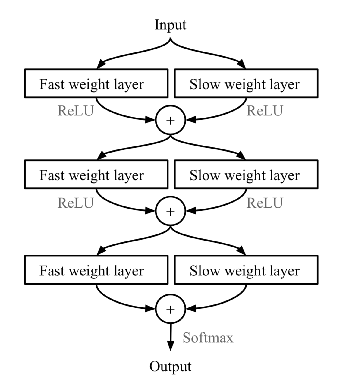
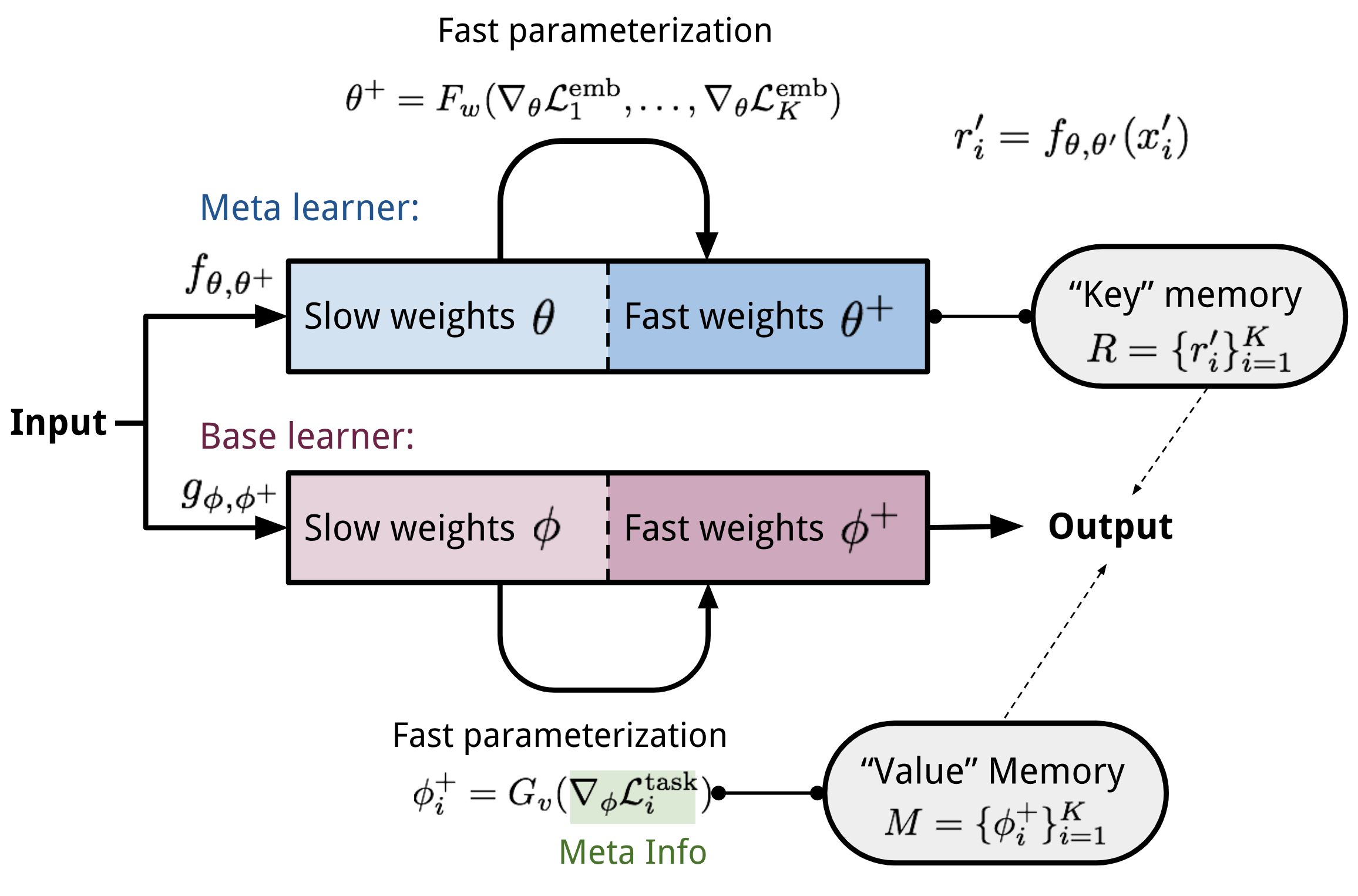
MetaNet’s rapid generalization depends on “fast weights”. Although there are several papers on this topic, I have not studied all of them in depth, and I was not able to find a single, precise definition. Instead, there seems to be a general, somewhat informal consensus around the idea. Typically, neural network weights are updated via stochastic gradient descent on an objective function, and this optimization process is known to be slow. A faster alternative is to use one neural network to predict the parameters of another neural network, and these generated parameters are referred to as fast weights. By contrast, the standard SGD-trained weights are called slow weights.
In MetaNet, loss gradients are treated as meta information and are used to drive models that generate fast weights. Predictions in the neural networks are then produced by combining slow and fast weights.
Model Components
Disclaimer: Below you will find my annotations are different from those in the paper. imo, the paper is poorly written, but the idea is still interesting. So I’m presenting the idea in my own language.
MetaNet consists of the following key components:
- An embedding function $f_\theta$, parameterized by $\theta$, which maps raw inputs to feature vectors. Similar to Siamese Neural Network, these embeddings are trained to be useful for determining whether two inputs belong to the same class (a verification task).
- A base learner $g_\phi$, parameterized by weights $\phi$, which performs the actual learning task.
If we stopped at this point, the setup would look identical to Relation Network. MetaNet additionally and explicitly models the fast weights for both functions, and then integrates them back into the overall model (see Fig. 8).
As a result, two additional functions are required to produce fast weights for $f$ and $g$, respectively.
- $F_w$: an LSTM parameterized by $w$ that learns fast weights $\theta^+$ for the embedding function $f$. Its input is the gradients of $f$’s embedding loss for the verification task.
- $G_v$: a neural network parameterized by $v$ that learns fast weights $\phi^+$ for the base learner $g$ from the learner’s loss gradients. In MetaNet, these loss gradients are treated as the task’s meta information.
Next, we consider how Meta Networks are trained. The training data consists of multiple dataset pairs: a support set $S=\{\mathbf{x}’_i, y’_i\}_{i=1}^K$ and a test set $U=\{\mathbf{x}_i, y_i\}_{i=1}^L$. Recall that there are four networks and four corresponding sets of parameters to learn, $(\theta, \phi, w, v)$.
Training Process
-
At each time step t, sample a random pair of inputs from the support set $S$, $(\mathbf{x}’_i, y’_i)$ and $(\mathbf{x}’_j, y_j)$. Let $\mathbf{x}_{(t,1)}=\mathbf{x}’_i$ and $\mathbf{x}_{(t,2)}=\mathbf{x}’_j$.
for $t = 1, \dots, K$:- a. Compute the representation-learning loss, for example cross entropy for the verification task:
$\mathcal{L}^\text{emb}_t = \mathbf{1}_{y’_i=y’_j} \log P_t + (1 - \mathbf{1}_{y’_i=y’_j})\log(1 - P_t)\text{, where }P_t = \sigma(\mathbf{W}\vert f_\theta(\mathbf{x}_{(t,1)}) - f_\theta(\mathbf{x}_{(t,2)})\vert)$
- a. Compute the representation-learning loss, for example cross entropy for the verification task:
-
Compute the task-level fast weights: $\theta^+ = F_w(\nabla_\theta \mathcal{L}^\text{emb}_1, \dots, \mathcal{L}^\text{emb}_T)$
-
Then iterate over examples in the support set $S$ to compute the example-level fast weights. At the same time, update the memory using the learned representations.
for $i=1, \dots, K$:- a. The base learner outputs a probability distribution: $P(\hat{y}_i \vert \mathbf{x}_i) = g_\phi(\mathbf{x}_i)$, and the loss can be cross-entropy or MSE: $\mathcal{L}^\text{task}_i = y’_i \log g_\phi(\mathbf{x}’_i) + (1- y’_i) \log (1 - g_\phi(\mathbf{x}’_i))$
- b. Extract the task’s meta information (loss gradients) and compute the example-level fast weights:
$\phi_i^+ = G_v(\nabla_\phi\mathcal{L}^\text{task}_i)$
- Then store $\phi^+_i$ into $i$-th location of the “value” memory $\mathbf{M}$.
- Then store $\phi^+_i$ into $i$-th location of the “value” memory $\mathbf{M}$.
- d. Encode the support sample into a task-specific input representation using both slow and fast weights: $r’_i = f_{\theta, \theta^+}(\mathbf{x}’_i)$
- Then store $r’_i$ into $i$-th location of the “key” memory $\mathbf{R}$.
-
Finally, construct the training loss using the test set $U=\{\mathbf{x}_i, y_i\}_{i=1}^L$.
Starts with $\mathcal{L}_\text{train}=0$:
for $j=1, \dots, L$:- a. Encode the test sample into a task-specific input representation: $r_j = f_{\theta, \theta^+}(\mathbf{x}_j)$
- b. Compute fast weights by attending to the support-set representations stored in memory $\mathbf{R}$. The attention function may be chosen freely; MetaNet uses cosine similarity here:
$ \begin{aligned} a_j &= \text{cosine}(\mathbf{R}, r_j) = [\frac{r'_1\cdot r_j}{\|r'_1\|\cdot\|r_j\|}, \dots, \frac{r'_N\cdot r_j}{\|r'_N\|\cdot\|r_j\|}]\\ \phi^+_j &= \text{softmax}(a_j)^\top \mathbf{M} \end{aligned} $- c. Update the training loss: $\mathcal{L}_\text{train} \leftarrow \mathcal{L}_\text{train} + \mathcal{L}^\text{task}(g_{\phi, \phi^+}(\mathbf{x}_i), y_i) $
-
Update all parameters $(\theta, \phi, w, v)$ using $\mathcal{L}_\text{train}$.
Optimization-Based
Deep learning models learn by backpropagating gradients. However, gradient-based optimization is not designed to perform well with only a small number of training samples, nor is it intended to converge in only a few optimization steps. Can we modify the optimization procedure so that a model becomes effective at learning from just a few examples? This is the objective of optimization-based meta-learning methods.
LSTM Meta-Learner
The optimization algorithm itself can be modeled explicitly. Ravi & Larochelle (2017) did this and referred to it as a “meta-learner”, while the original model used to solve the task is called the “learner”. The meta-learner’s goal is to update the learner’s parameters efficiently from a small support set, enabling rapid adaptation to a new task.
Let the learner be $M_\theta$ with parameters $\theta$, the meta-learner be $R_\Theta$ with parameters $\Theta$, and the loss function be $\mathcal{L}$.
Why LSTM?
The meta-learner is implemented as an LSTM for two reasons:
- Gradient-based updates in backpropagation resemble the LSTM cell-state update.
- Having access to a history of gradients can improve the update rule, similar to how momentum operates.
The learner’s parameter update at time step t, with learning rate $\alpha_t$, is:
This has the same structure as the LSTM cell-state update if we map the forget gate to $f_t=1$, the input gate to $i_t = \alpha_t$, the cell state to $c_t = \theta_t$, and the new cell state to $\tilde{c}_t = -\nabla_{\theta_{t-1}}\mathcal{L}_t$:
Although fixing $f_t=1$ and $i_t=\alpha_t$ may not be optimal, both can instead be learned and adapted to different datasets.
Model Setup
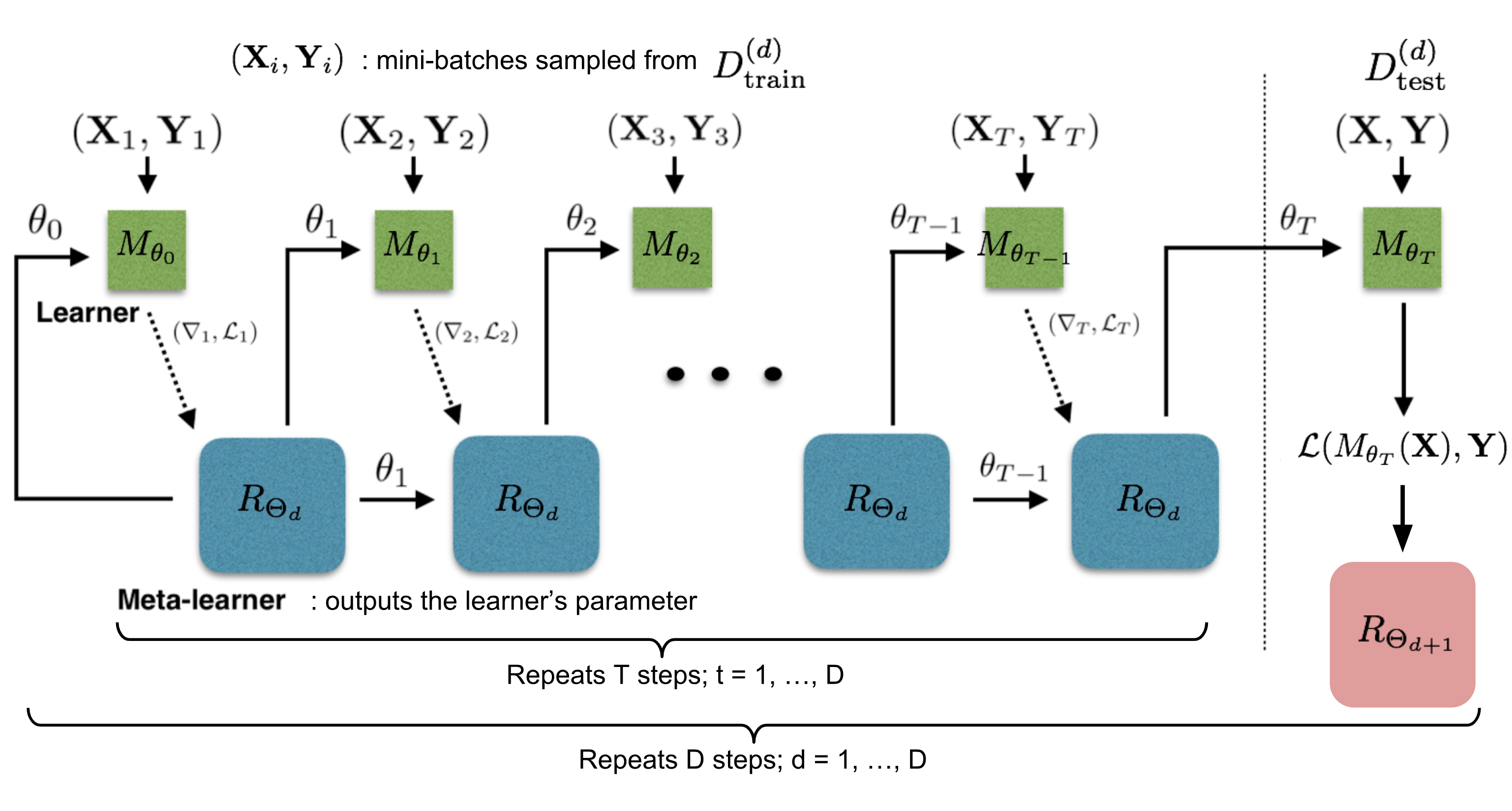
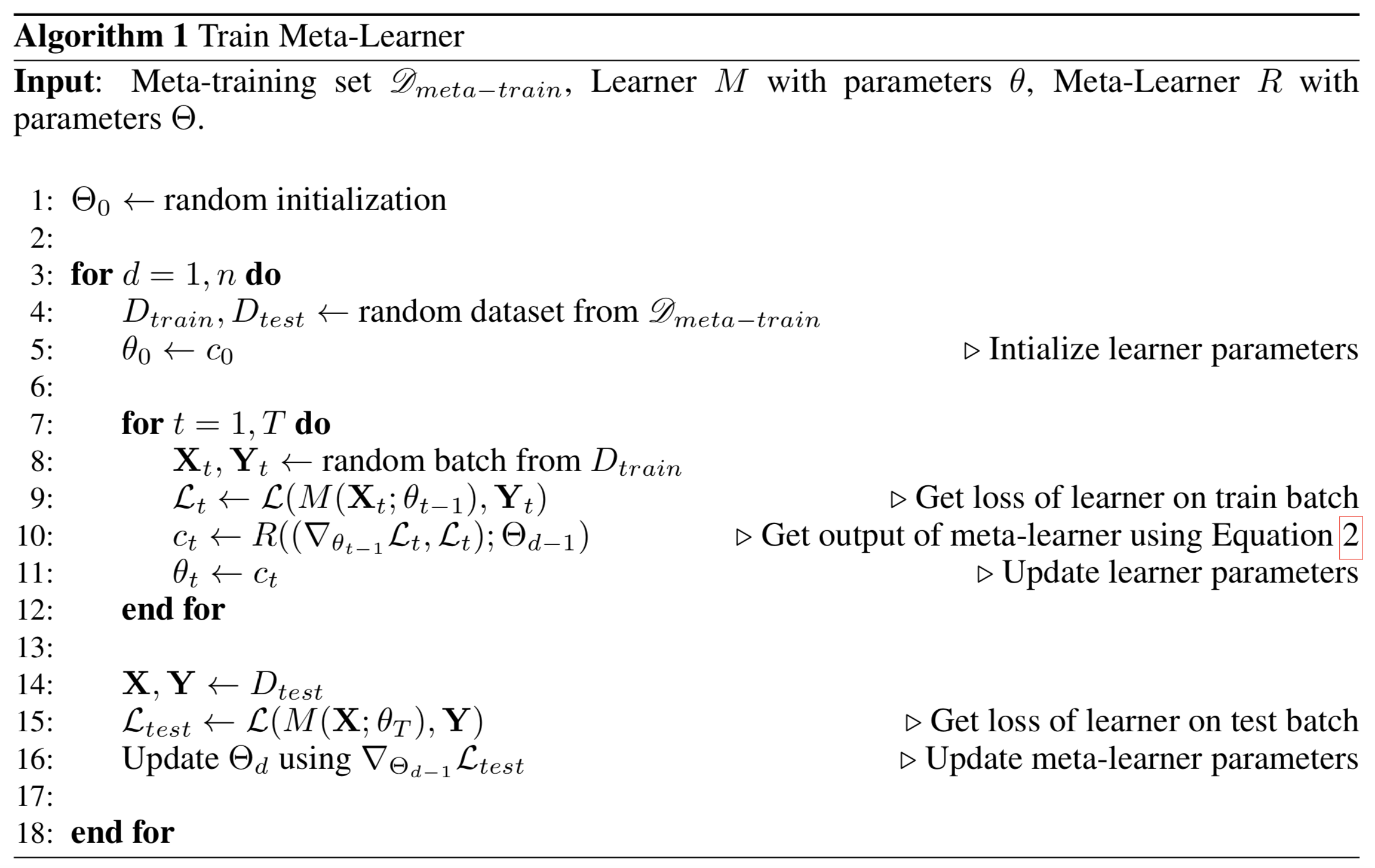
The training procedure mirrors test-time behavior, since this has been shown to be beneficial in Matching Networks. In each training epoch, we first sample a dataset $\mathcal{D} = (\mathcal{D}_\text{train}, \mathcal{D}_\text{test}) \in \hat{\mathcal{D}}_\text{meta-train}$, then draw mini-batches from $\mathcal{D}_\text{train}$ to update $\theta$ for $T$ rounds. The learner’s final parameter state $\theta_T$ is then used to train the meta-learner on the test data $\mathcal{D}_\text{test}$.
Two implementation details deserve special attention:
- How should the parameter space be compressed in an LSTM meta-learner? Because the meta-learner models the parameters of another neural network, it would otherwise need to learn hundreds of thousands of variables. Following the idea approach of sharing parameters across coordinates,
- To simplify training, the meta-learner assumes that the loss $\mathcal{L}_t$ and the gradient $\nabla_{\theta_{t-1}} \mathcal{L}_t$ are independent.
MAML
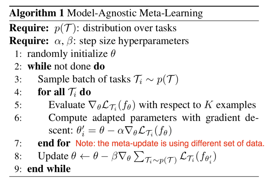
MAML, short for Model-Agnostic Meta-Learning (Finn, et al. 2017), is a broadly applicable optimization algorithm that can be used with any model trained via gradient descent.
Suppose our model is $f_\theta$ with parameters $\theta$. Given a task $\tau_i$ and its corresponding dataset $(\mathcal{D}^{(i)}_\text{train}, \mathcal{D}^{(i)}_\text{test})$, we can update the model parameters using one or more gradient descent steps (the example below shows a single step):
where $\mathcal{L}^{(0)}$ is the loss computed on the mini data batch with id (0).
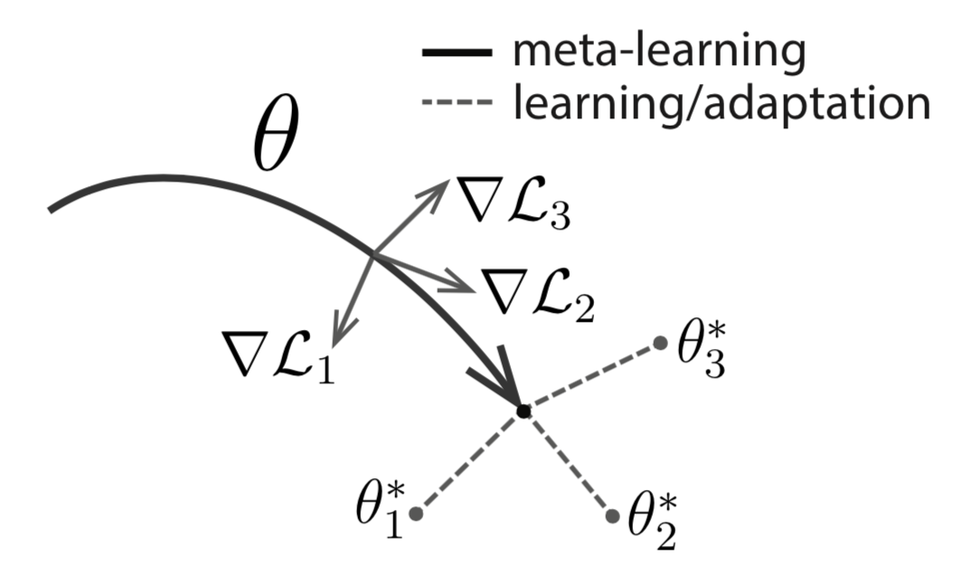
However, the formula above optimizes only for a single task. To generalize well across a range of tasks, we want to find an optimal $\theta^*$ such that task-specific fine-tuning becomes more efficient. To do this, we sample a new data batch with id (1) to update the meta-objective. The loss, denoted $\mathcal{L}^{(1)}$, depends on mini batch (1). The superscripts in $\mathcal{L}^{(0)}$ and $\mathcal{L}^{(1)}$ merely indicate different data batches, and they refer to the same loss objective for the same task.
First-Order MAML
The meta-optimization step above depends on second derivatives. To reduce computational cost, a modified version of MAML drops the second-derivative terms, yielding a simpler and less expensive implementation known as First-Order MAML (FOMAML).
Consider performing $k$ inner gradient steps, $k\geq1$. Starting from the initial model parameter $\theta_\text{meta}$:
Then, in the outer loop, we sample a new data batch to update the meta-objective.
The MAML gradient is:
First-Order MAML ignores the second-derivative component shown in red. This yields the following simplification, which is equivalent to taking the derivative of the final inner-gradient update result:
Reptile
Reptile (Nichol, Achiam & Schulman, 2018) is an exceptionally simple meta-learning optimization algorithm. In many respects, it resembles MAML, since both methods perform meta-optimization with gradient descent and both are model-agnostic.
Reptile repeatedly does the following:
- sample a task,
- train on it using multiple gradient descent steps,
- move the model weights toward the newly obtained parameters.
See the algorithm below: $\text{SGD}(\mathcal{L}_{\tau_i}, \theta, k)$ performs a stochastic gradient update for k steps on the loss $\mathcal{L}_{\tau_i}$, starting from the initial parameter $\theta$, and returns the final parameter vector. The batch version samples multiple tasks, rather than one, in each iteration. The Reptile gradient is defined as $(\theta - W)/\alpha$, where $\alpha$ is the stepsize used by the SGD operation.
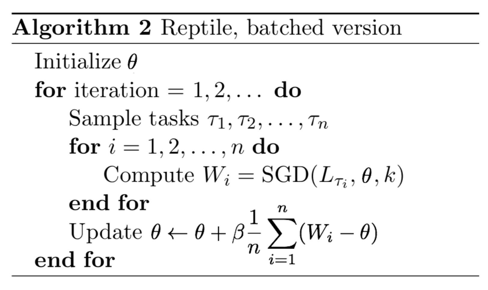
At first glance, the procedure resembles ordinary SGD. However, because task-specific optimization can involve more than one step, it eventually causes $\text{SGD}(\mathbb{E} _\tau[\mathcal{L}_{\tau}], \theta, k)$ to diverge from $\mathbb{E}_\tau [\text{SGD}(\mathcal{L}_{\tau}, \theta, k)]$ when k > 1.
The Optimization Assumption
Assume a task $\tau \sim p(\tau)$ has a manifold of optimal network configurations, $\mathcal{W}_{\tau}^*$. The model $f_\theta$ achieves the best performance for task $\tau$ when $\theta$ lies on the surface of $\mathcal{W}_{\tau}^*$. To obtain a solution that performs well across tasks, we would like to find a parameter that is close to the optimal manifolds of all tasks:
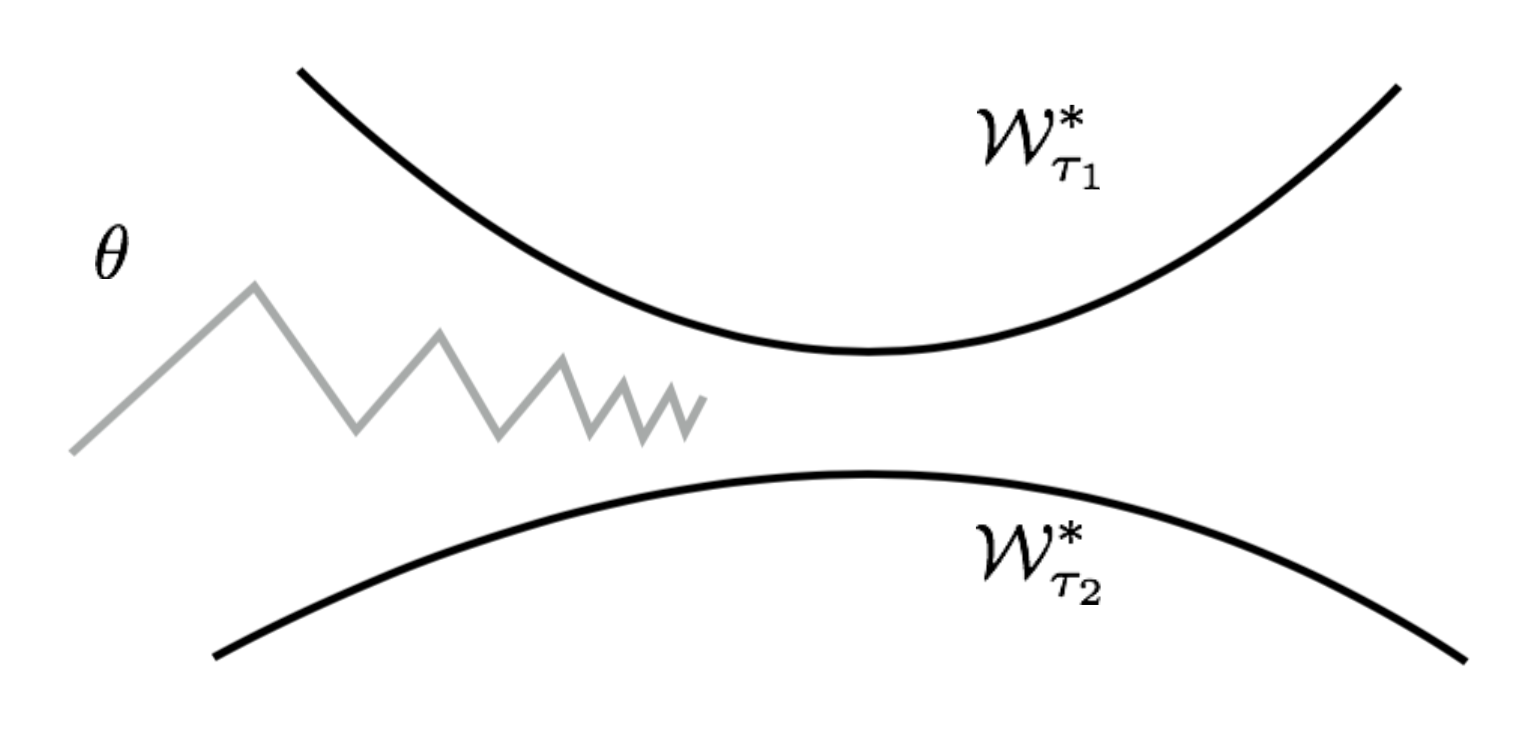
Let us use the L2 distance as $\text{dist}(.)$. The distance between a point $\theta$ and a set $\mathcal{W}_\tau^*$ is equal to the distance between $\theta$ and the point $W_{\tau}^*(\theta)$ on the manifold that is closest to $\theta$:
The gradient of the squared Euclidean distance is:
Notes: According to the Reptile paper, “the gradient of the squared euclidean distance between a point $\Theta$ and a set $S$ is the vector $2(\Theta − p)$, where p is the closest point in $S$ to $\Theta$”. Technically, the closest point in $S$ is also a function of $\Theta$, but I am not sure why the gradient does not need to consider the derivative of $p$. (Please feel free to leave me a comment or send me an email about this if you have ideas.)
Therefore, the update rule for one stochastic gradient step is:
The closest point on the optimal task manifold $W_{\tau_i}^*(\theta)$ cannot be computed exactly, but Reptile approximates it using $\text{SGD}(\mathcal{L}_\tau, \theta, k)$.
Reptile vs FOMAML
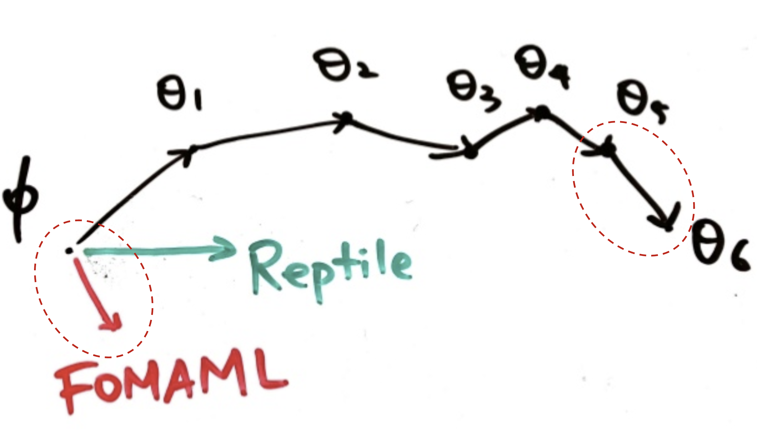
To illustrate the deeper connection between Reptile and MAML, let us expand the update formula using an example with two gradient steps, k=2 in $\text{SGD}(.)$. As defined in above, $\mathcal{L}^{(0)}$ and $\mathcal{L}^{(1)}$ are losses computed from different mini-batches of data. For readability, we use two simplified notations: $g^{(i)}_j = \nabla_{\theta} \mathcal{L}^{(i)}(\theta_j)$ and $H^{(i)}_j = \nabla^2_{\theta} \mathcal{L}^{(i)}(\theta_j)$.
According to early section, the gradient of FOMAML is the result of the final inner-gradient update. Therefore, when k=1:
The Reptile gradient is defined as:
Up to this point, we have:
Next, let us expand $g^{(1)}_1$ further using Taylor expansion. Recall that the Taylor expansion of a function $f(x)$ that is differentiable at a number $a$ is:
We can treat $\nabla_{\theta}\mathcal{L}^{(1)}(.)$ as a function and $\theta_0$ as an input value. The Taylor expansion of $g_1^{(1)}$ at the value point $\theta_0$ is:
Substitute the expanded form of $g_1^{(1)}$ into the MAML gradients with a one-step inner-gradient update:
The Reptile gradient then becomes:
At this stage, we have expressions for three types of gradients:
During training, we often average across multiple data batches. In this example, mini batches (0) and (1) are interchangeable because both are randomly sampled. The expectation $\mathbb{E}_{\tau,0,1}$ is averaged over the two data batches, ids (0) and (1), for task $\tau$.
Let:
- $A = \mathbb{E}_{\tau,0,1} [g_0^{(0)}] = \mathbb{E}_{\tau,0,1} [g_0^{(1)}]$; this is the average gradient of the task loss. We aim to improve the model parameters to achieve better task performance by following the direction indicated by $A$.
- $B = \mathbb{E}_{\tau,0,1} [H^{(1)}_0 g_0^{(0)}] = \frac{1}{2}\mathbb{E}_{\tau,0,1} [H^{(1)}_0 g_0^{(0)} + H^{(0)}_0 g_0^{(1)}] = \frac{1}{2}\mathbb{E}_{\tau,0,1} [\nabla_\theta(g^{(0)}_0 g_0^{(1)})]$; this is the direction (gradient) that increases the inner product of gradients from two different mini batches for the same task. We aim to improve the model parameters to achieve better generalization across different data by following the direction indicated by $B$.
In conclusion, both MAML and Reptile attempt to optimize the same objective, improved task performance (guided by A) and improved generalization (guided by B), when the gradient update is approximated by the first three leading terms.
It is not clear to me whether the omitted term $O(\alpha^2)$ could have a substantial impact on parameter learning. However, given that FOMAML can achieve performance similar to the full version of MAML, it may be reasonable to infer that higher-order derivatives are not critical during gradient descent updates.
Cited as:
@article{weng2018metalearning,
  title   = "Meta-Learning: Learning to Learn Fast",
  author  = "Weng, Lilian",
  journal = "lilianweng.github.io",
  year    = "2018",
  url     = "https://lilianweng.github.io/posts/2018-11-30-meta-learning/"
}
Reference
[1] Brenden M. Lake, Ruslan Salakhutdinov, and Joshua B. Tenenbaum. “Human-level concept learning through probabilistic program induction.” Science 350.6266 (2015): 1332-1338.
[2] Oriol Vinyals’ talk on “Model vs Optimization Meta Learning”
[3] Gregory Koch, Richard Zemel, and Ruslan Salakhutdinov. “Siamese neural networks for one-shot image recognition.” ICML Deep Learning Workshop. 2015.
[4] Oriol Vinyals, et al. “Matching networks for one shot learning.” NIPS. 2016.
[5] Flood Sung, et al. “Learning to compare: Relation network for few-shot learning.” CVPR. 2018.
[6] Jake Snell, Kevin Swersky, and Richard Zemel. “Prototypical Networks for Few-shot Learning.” CVPR. 2018.
[7] Adam Santoro, et al. “Meta-learning with memory-augmented neural networks.” ICML. 2016.
[8] Alex Graves, Greg Wayne, and Ivo Danihelka. “Neural turing machines.” arXiv preprint arXiv:1410.5401 (2014).
[9] Tsendsuren Munkhdalai and Hong Yu. “Meta Networks.” ICML. 2017.
[10] Sachin Ravi and Hugo Larochelle. “Optimization as a Model for Few-Shot Learning.” ICLR. 2017.
[11] Chelsea Finn’s BAIR blog on “Learning to Learn”.
[12] Chelsea Finn, Pieter Abbeel, and Sergey Levine. “Model-agnostic meta-learning for fast adaptation of deep networks.” ICML 2017.
[13] Alex Nichol, Joshua Achiam, John Schulman. “On First-Order Meta-Learning Algorithms.” arXiv preprint arXiv:1803.02999 (2018).
[14] Slides on Reptile by Yoonho Lee.