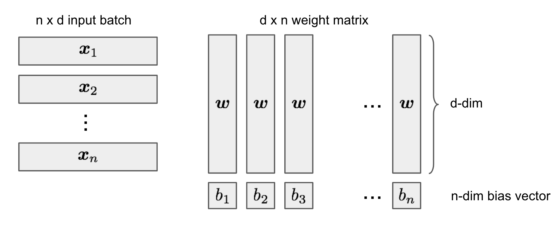
Given $a_i = \boldsymbol{x}_i \boldsymbol{w}$, our goal is to choose appropriate $\boldsymbol{w}$ and $\boldsymbol{b}$ such that $b_1 < a_1 < b_2 < a_2 < \dots < b_n < a_n$ holds. This is always possible because we are solving $n+d$ unknown variables under $n$ constraints, and $\boldsymbol{x}_i$ are independent (for example, choose a random $\boldsymbol{w}$, sort $\boldsymbol{x}_i \boldsymbol{w}$, and then assign the $b_j$’s to be intermediate values). Under this construction, $\mathbf{M}_\text{ReLU}$ becomes a lower triangular matrix:

This matrix is a nonsingular square matrix because $\det(\mathbf{M}_\text{ReLU}) \neq 0$, so we can always find suitable $\boldsymbol{v}$ to solve $\boldsymbol{v}\mathbf{M}_\text{ReLU}=\boldsymbol{y}$. Equivalently, the column space of $\mathbf{M}_\text{ReLU}$ is the entirety of $\mathbb{R}^n$, and we can form any $\boldsymbol{y}$ as a linear combination of its column vectors.

Deep NN can Learn Random Noise

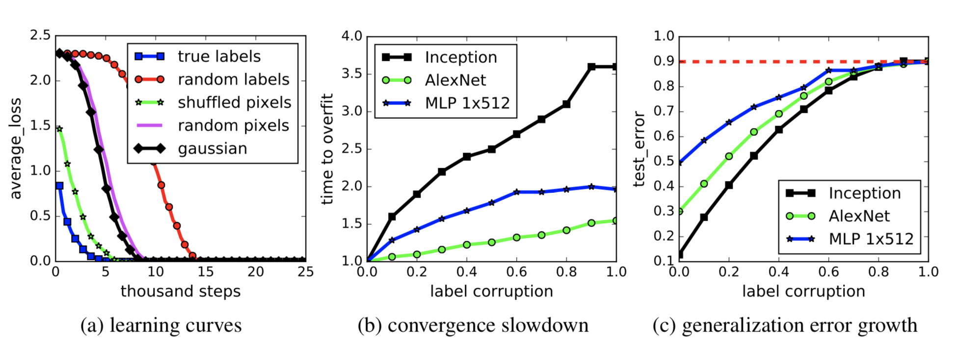
Because two-layer neural networks are universal approximators, it is not especially surprising that they can fit unstructured random noise perfectly, as demonstrated in Zhang, et al. (2017). When the labels in an image classification dataset are randomly permuted, the high expressive capacity of deep neural networks still enables them to drive the training loss close to zero. Notably, these findings remain qualitatively unchanged even when regularization terms are added.

Are Deep Learning Models Dramatically Overfitted?

Deep learning models are often heavily over-parameterized and can frequently achieve perfect performance on the training set. From the traditional perspective (for example, the bias-variance trade-off), this would appear disastrous, suggesting that the model might fail to generalize to unseen test data. Yet, in practice, these seemingly “overfitted” deep models (training error = 0) often still deliver solid out-of-sample performance. This raises a natural question: why does this happen?

Modern Risk Curve for Deep Learning

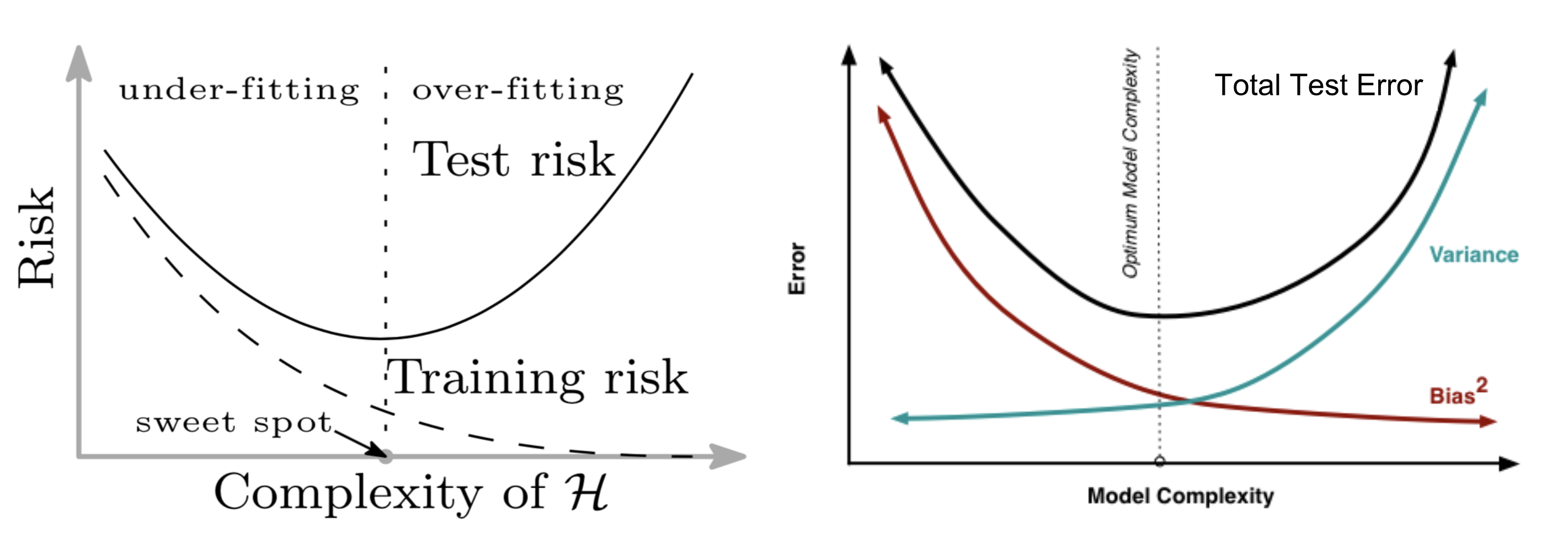
Traditional machine learning commonly relies on a U-shaped risk curve to characterize the bias-variance trade-off and to quantify how well a model is expected to generalize. If asked how to identify whether a model is overfitted, this is typically the first diagnostic that comes to mind.

As the model grows (that is, as more parameters are added), training error tends to fall toward zero. However, once model complexity crosses the boundary between “underfitting” and “overfitting,” the test error (generalization error) begins to rise. In spirit, this is consistent with Occam’s Razor.

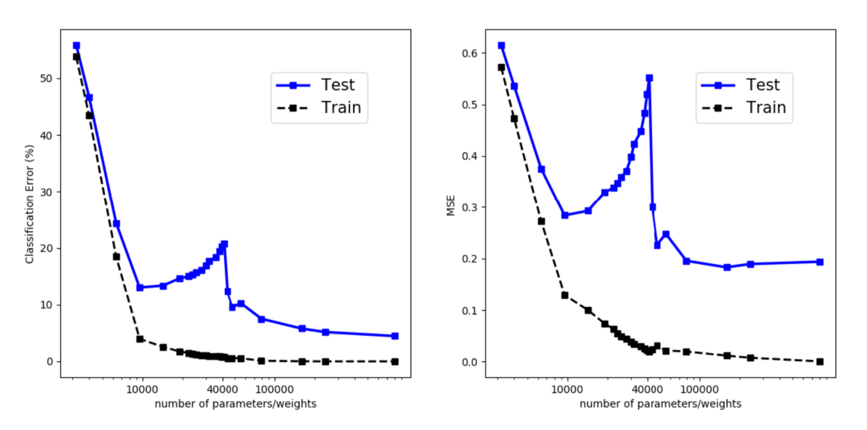
However, this picture does not cleanly describe deep learning. Belkin et al. (2018) reconciled the classical bias-variance framing with modern behavior by proposing a new double-U-shaped risk curve for deep neural networks. In their view, once a network has sufficiently many parameters, the risk curve transitions into an additional regime.

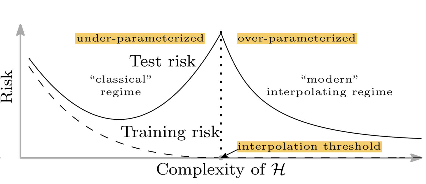
The paper argued that this behavior is likely driven by two factors:

• The parameter count is a poor proxy for inductive bias, which is defined as the set of assumptions a learning algorithm uses to make predictions on previously unseen samples. For additional discussion of deep learning model complexity, see the later sections.
• With a larger model, we may be able to explore broader function classes and identify interpolating functions with smaller norms, and therefore “simpler” solutions.

The double-U-shaped curve was reported empirically in the paper. That said, I found it fairly challenging to reproduce. While there are encouraging signs, producing a smooth curve comparable to the theorem requires careful control of many details in the experimental setup.

Regularization is not the Key to Generalization

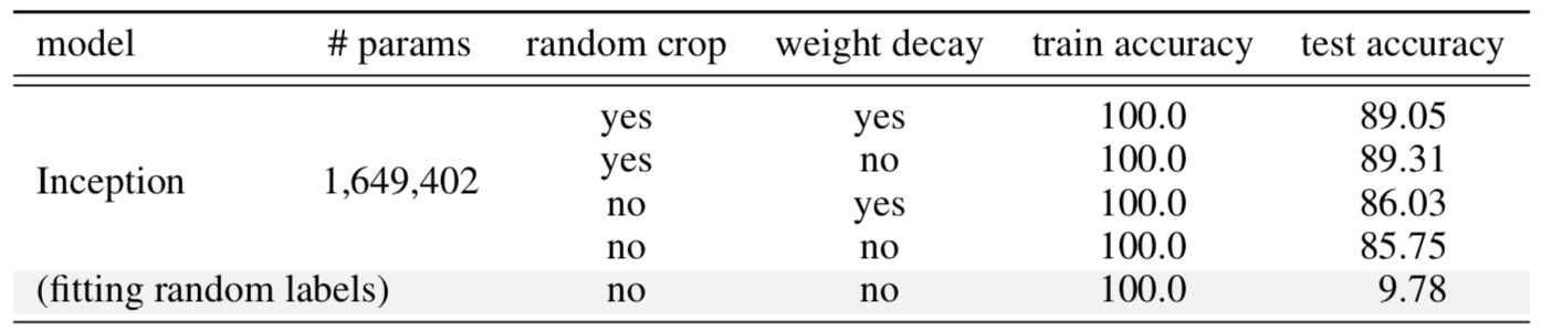
Regularization is a standard tool for controlling overfitting and improving generalization. Interestingly, some work (Zhang, et al. 2017) suggests that explicit regularization (for example, data augmentation, weight decay, and dropout) is neither necessary nor sufficient to reduce generalization error.

Using an Inception model trained on CIFAR10 as an example (see Fig. 5), regularization methods help out-of-sample generalization, but not dramatically. No single regularization component appears essential in isolation from the others. Therefore, it seems unlikely that regularizers are the fundamental reason deep models generalize.

Intrinsic Dimension

In deep learning, parameter count often fails to correlate with overfitting, indicating that counting parameters does not capture the true complexity of deep neural networks.

Beyond parameter counting, many alternative complexity measures have been proposed, including the number of degrees of freedom of models (Gao & Jojic, 2016) and prequential code (Blier & Ollivier, 2018).

Here, I focus on a more recent approach called intrinsic dimension (Li et al, 2018). Intrinsic dimension is conceptually straightforward, relatively easy to measure, and it reveals notable properties across models of different sizes.

Consider a neural network with a very large number of parameters, which defines a high-dimensional parameter space. Learning then proceeds over this high-dimensional objective landscape. The geometry of the parameter-space manifold is important. For instance, a smoother manifold can make optimization easier by providing more predictive gradients and permitting larger learning rates, which was proposed as a reason batch normalization can stabilize training (Santurkar, et al, 2019).

Although the parameter space is enormous, we do not necessarily need to worry that optimization will be trapped in poor local optima. It has been shown that local optimal points in the objective landscape almost always occur at saddle points rather than true valleys. Put differently, there is typically a subset of dimensions that provides directions to escape and continue exploring.

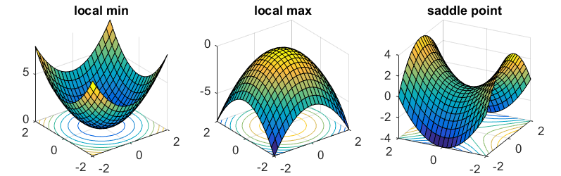
A key intuition behind intrinsic dimension is that, in such a high-dimensional parameter space, effective learning may not require using every dimension. If optimization can move through only a slice of the objective landscape and still reach a strong solution, then the effective complexity of the resulting model may be far smaller than parameter counting would suggest. Intrinsic dimension is designed to quantify this notion.

Suppose a model has $D$ dimensions, with parameters denoted by $\theta^{(D)}$. For training, we randomly sample a smaller $d$-dimensional subspace, $\theta^{(d)}$, where $d < D$. During each optimization update, instead of taking a gradient step in all $D$ dimensions, we update only within the smaller subspace $\theta^{(d)}$ and then remap that update back to the full parameter space.

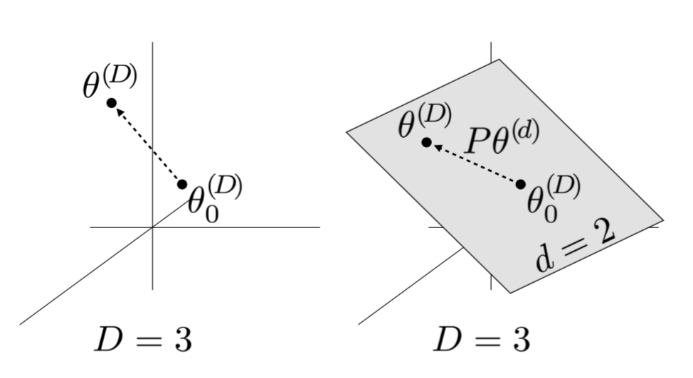
The gradient update takes the following form:

where $\theta_0^{(D)}$ are the initialization values and $\mathbf{P}$ is a $D \times d$ projection matrix sampled at random prior to training. Both $\theta_0^{(D)}$ and $\mathbf{P}$ are fixed (not trainable) throughout training. $\theta^{(d)}$ is initialized to all zeros.

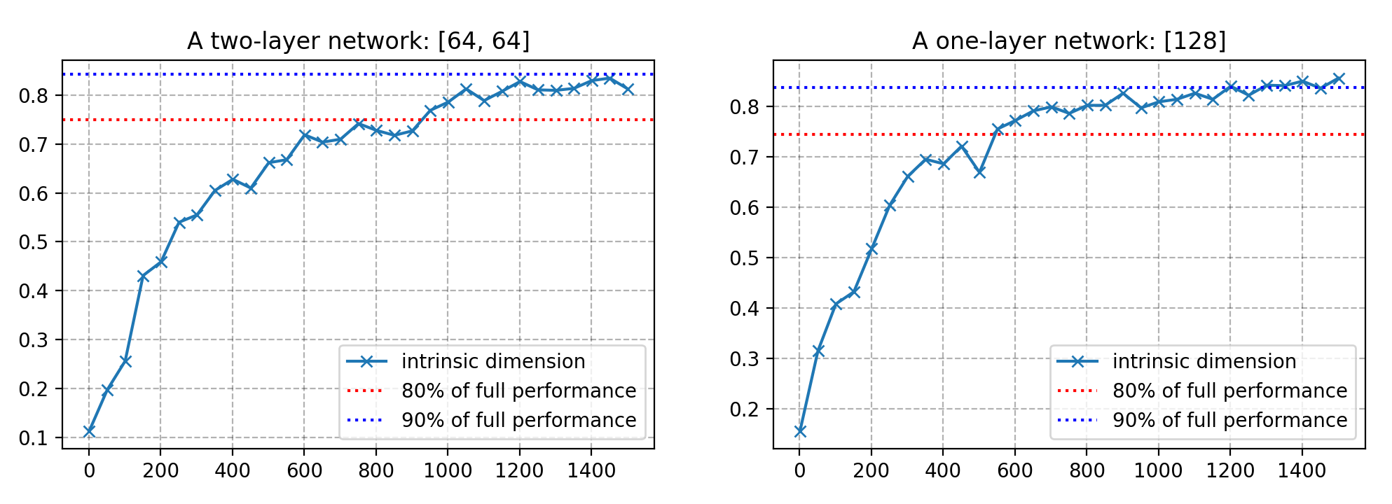
By searching over $d = 1, 2, \dots, D$, the associated $d$ at which a solution first appears is defined as the intrinsic dimension.

Empirically, many tasks exhibit intrinsic dimensions far smaller than their raw parameter counts. For instance, in CIFAR10 image classification, a fully connected network with 650k+ parameters has an intrinsic dimension of only 9k, and a convolutional network with 62k parameters has an even lower intrinsic dimension of 2.9k.

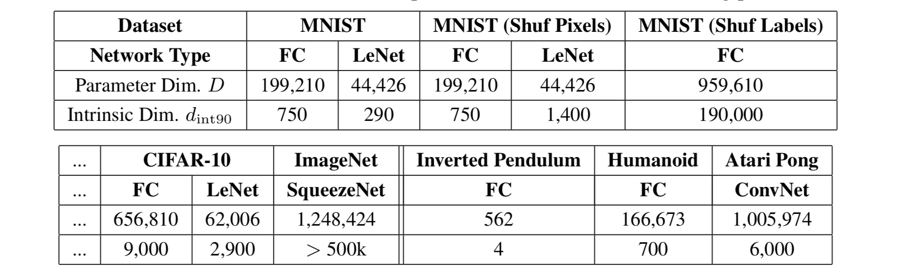
These intrinsic-dimension measurements suggest that deep learning models can be substantially simpler than they appear based solely on parameter counts.

Heterogeneous Layer Robustness

Zhang et al. (2019) studied how parameters in different layers contribute to model behavior. Their central question is: “are all layers created equal?” Their conclusion is that they are not, some layers are much more sensitive to perturbations than others.

The paper introduced two parameter interventions for the $\ell$-th layer, $\ell = 1, \dots, L$, at time $t$, $\theta^{(\ell)}_t$, and examined their effects on robustness:

• Re-initialization: Reset the layer parameters to their initialization values, $\theta^{(\ell)}_t \leftarrow \theta^{(\ell)}_0$. The resulting network performance after re-initializing layer $\ell$ is called the re-initialization robustness of layer $\ell$.

• Re-randomization: Resample the layer parameters at random, $\theta^{(\ell)}_t \leftarrow \tilde{\theta}^{(\ell)} \sim \mathcal{P}^{(\ell)}$. The resulting network performance is called the re-randomization robustness of layer $\ell$.

Using these two operations, layers can be grouped into two types:

• Robust Layers: Re-initializing or re-randomizing the layer causes no, or only negligible, degradation in performance.
• Critical Layers: Any layer that does not satisfy the robust criterion.

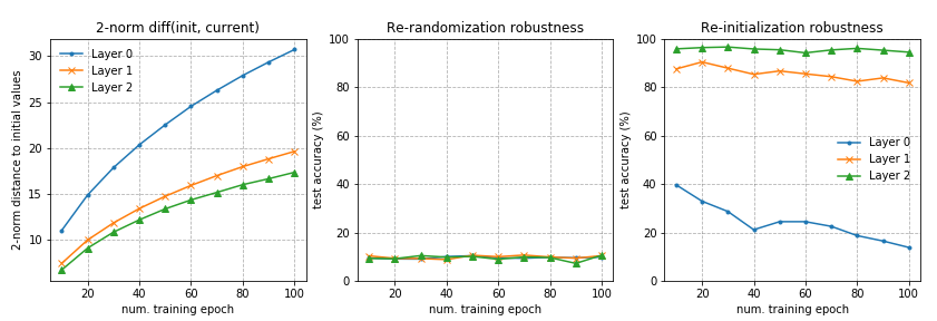
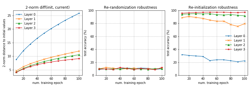
Comparable patterns appear in both fully connected and convolutional networks. Re-randomizing any layer completely destroys performance, with predictions immediately collapsing to random guessing. More unexpectedly, under re-initialization, only the first layer or the first few layers (closest to the input) are critical, while re-initializing higher layers produces only negligible decrease in performance.

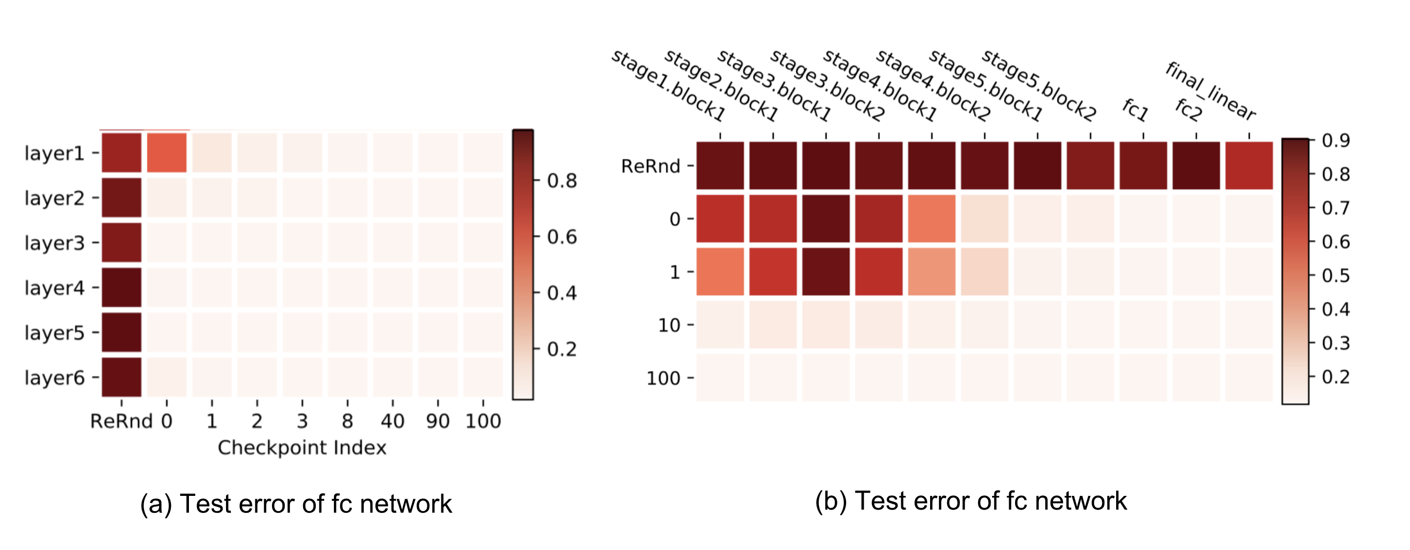
ResNet can leverage shortcut connections between non-adjacent layers, redistributing sensitivity across the network rather than concentrating it near the bottom. With residual blocks, the network can evenly be robust to re-randomization. Only the first layer in each residual block remains sensitive to both re-initialization and re-randomization. If each residual block is treated as a local sub-network, the robustness pattern resembles what is observed for the fully connected and convolutional networks above.

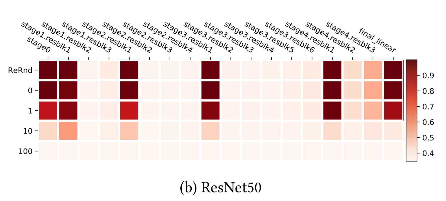
Because many upper layers in deep networks are not critical to performance under re-initialization, the paper offered the following loose conclusion:

“Over-capacitated deep networks trained with stochastic gradient have low-complexity due to self-restricting the number of critical layers.”

Re-initialization can be interpreted as a mechanism for reducing the effective number of parameters. In that sense, this observation is consistent with what intrinsic dimension suggests.

The Lottery Ticket Hypothesis

The lottery ticket hypothesis (Frankle & Carbin, 2019) provides another compelling result supporting the idea that only a subset of parameters materially determines performance, and therefore the network is not necessarily overfitted in the intuitive sense. The hypothesis proposes that a randomly initialized, dense, feed-forward network contains many subnetworks, and that only some of these subnetworks are “winning tickets” capable of reaching optimal performance when trained in isolation.

This idea is motivated by network pruning methods, which remove unnecessary weights (for example, very small weights that contribute negligibly) without reducing accuracy. Although pruning can drastically reduce the final model size, training the resulting pruned architecture successfully from scratch is difficult. This creates an apparent tension: training seems to benefit from many parameters, but maintaining high accuracy after training does not require nearly as many. Why?

To study this, the lottery ticket hypothesis conducted the following procedure:

1. Randomly initialize a dense feed-forward network with initialization values $\theta_0$;
2. Train the network for multiple iterations until it reaches good performance, yielding parameter configuration $\theta$;
3. Prune $\theta$, producing a mask $m$.
4. The “winning ticket” initialization configuration is $m \odot \theta_0$.

If we then train only the small “winning ticket” subset of parameters, using the same initial values found in step 1, the model can reach the same accuracy achieved in step 2. The implication is that a large parameter space may not be required to represent the final solution, but it can be useful during training because it supplies a large pool of initialization configurations for many much smaller subnetworks.

The lottery ticket hypothesis offers a new perspective for interpreting and dissecting deep neural network behavior, and it has inspired many follow-up studies.

Experiments

After reviewing the findings above, reproducing them is an appealing exercise. Some results are easier to replicate than others, and the details are provided below. The code is available on github at lilianweng/generalization-experiment.

New Risk Curve for DL Models

This is the most difficult result to replicate. The authors shared several helpful suggestions, which I greatly appreciate. The following experimental settings are particularly important:

• No regularization is used (for example, no weight decay and no dropout).
• In Fig 3, the training set consists of 4k samples. It is sampled once and then held fixed across all models. Evaluation uses the full MNIST test set.
• Each network is trained for a long time to drive training risk close to zero. The learning rate is adjusted differently for models of different sizes.
• To reduce sensitivity to initialization in the under-parameterized regime, they employ a “weight reuse” scheme: parameters learned by a smaller network are used to initialize larger networks.

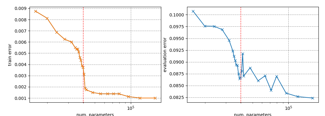
I did not train or tune each model long enough to reach perfect training performance, but the evaluation error does exhibit a distinctive twist around the interpolation threshold that differs from the training error. For MNIST, for example, the threshold equals the number of training samples multiplied by the number of classes (10), that is 40000.

The x-axis is the number of model parameters, computed as: (28 * 28 + 1) * num. units + num. units * 10, plotted on a logarithmic scale.

Layers are not Created Equal

This result is relatively straightforward to reproduce. See my implementation here.

In the first experiment, I used a three-layer fully connected network with 256 units per layer. Layer 0 is the input layer, and layer 3 is the output layer. The network is trained on MNIST for 100 epochs.

In the second experiment, I used a four-layer fully connected network with 128 units per layer. All other settings match experiment 1.

Intrinsic Dimension Measurement

To correctly map the $d$-dimensional subspace into the full parameter space, the projection matrix $\mathbf{P}$ should have orthogonal columns. Because the product $\mathbf{P}\theta^{(d)}$ is a sum of the columns of $\mathbf{P}$, each scaled by the corresponding scalar entry in the $d$-dimensional vector $\sum_{i=1}^d \theta^{(d)}_i \mathbf{P}^\top_{(:,i)}$, it is preferable to fully utilize the subspace by ensuring orthogonal columns in $\mathbf{P}$.

My implementation uses a naive approach: it samples a large matrix with independent entries from a standard normal distribution. In a high-dimensional space, the columns are expected to be independent and therefore approximately orthogonal. This approach works when the dimension is not too large. When experimenting with large $d$, sparse projection matrix constructions are available, which is what the intrinsic dimension paper recommended.

Below are experiment runs for two networks: (left) a two-layer fully connected network with 64 units in each layer, and (right) a one-layer fully connected network with 128 hidden units, trained on 10% of MNIST. For each $d$, the model is trained for 100 epochs. See the code here.

---

Cited as:

@article{weng2019overfit,
  title   = "Are Deep Neural Networks Dramatically Overfitted?",
  author  = "Weng, Lilian",
  journal = "lilianweng.github.io",
  year    = "2019",
  url     = "https://lilianweng.github.io/posts/2019-03-14-overfit/"
}

References

[1] Wikipedia page on Occam’s Razor.

[2] Occam’s Razor on Principia Cybernetica Web.

[3] Peter Grunwald. “A Tutorial Introduction to the Minimum Description Length Principle”. 2004.

[4] Ian Goodfellow, et al. Deep Learning. 2016. Sec 6.4.1.

[5] Zhang, Chiyuan, et al. “Understanding deep learning requires rethinking generalization.” ICLR 2017.

[6] Shibani Santurkar, et al. “How does batch normalization help optimization?.” NIPS 2018.

[7] Mikhail Belkin, et al. “Reconciling modern machine learning and the bias-variance trade-off.” arXiv:1812.11118, 2018.

[8] Chiyuan Zhang, et al. “Are All Layers Created Equal?” arXiv:1902.01996, 2019.

[9] Chunyuan Li, et al. “Measuring the intrinsic dimension of objective landscapes.” ICLR 2018.

[10] Jonathan Frankle and Michael Carbin. “The lottery ticket hypothesis: Finding sparse, trainable neural networks.” ICLR 2019.