Meta Reinforcement Learning
In my earlier post on meta-learning, I framed the problem primarily in the context of few-shot classification. Here, I would like to examine scenarios in which we aim to “meta-learn” Reinforcement Learning (RL) tasks by building an agent that can solve previously unseen tasks quickly and efficiently.
· 22 min read · Curated and presented by Arthur Sedek
In my earlier post on meta-learning, the problem is primarily framed in the setting of few-shot classification. Here, I would like to dig deeper into scenarios where we attempt to “meta-learn” Reinforcement Learning (RL) tasks by building an agent that can solve unseen tasks quickly and efficiently.
As a reminder, a strong meta-learning model should generalize to new tasks or environments that were never encountered during training. The adaptation process, essentially a mini learning session, occurs at test time with only limited exposure to the new configuration. Even without any explicit fine-tuning (no gradient backpropagation on trainable variables), the meta-learning model can autonomously adjust its internal hidden states in order to learn.
Training RL algorithms can be notoriously difficult. If a meta-learning agent became sufficiently capable that the set of solvable unseen tasks expanded to be extremely broad, we would be moving toward general purpose methods, essentially building a “brain” that could solve many kinds of RL problems with minimal human intervention or manual feature engineering. Sounds amazing, right? 💖
On the Origin of Meta-RL
Back in 2001
I came across a paper written in 2001 by Hochreiter et al. while reading Wang et al., 2016. Although the original proposal targets supervised learning, it has many parallels with modern approaches to meta-RL.
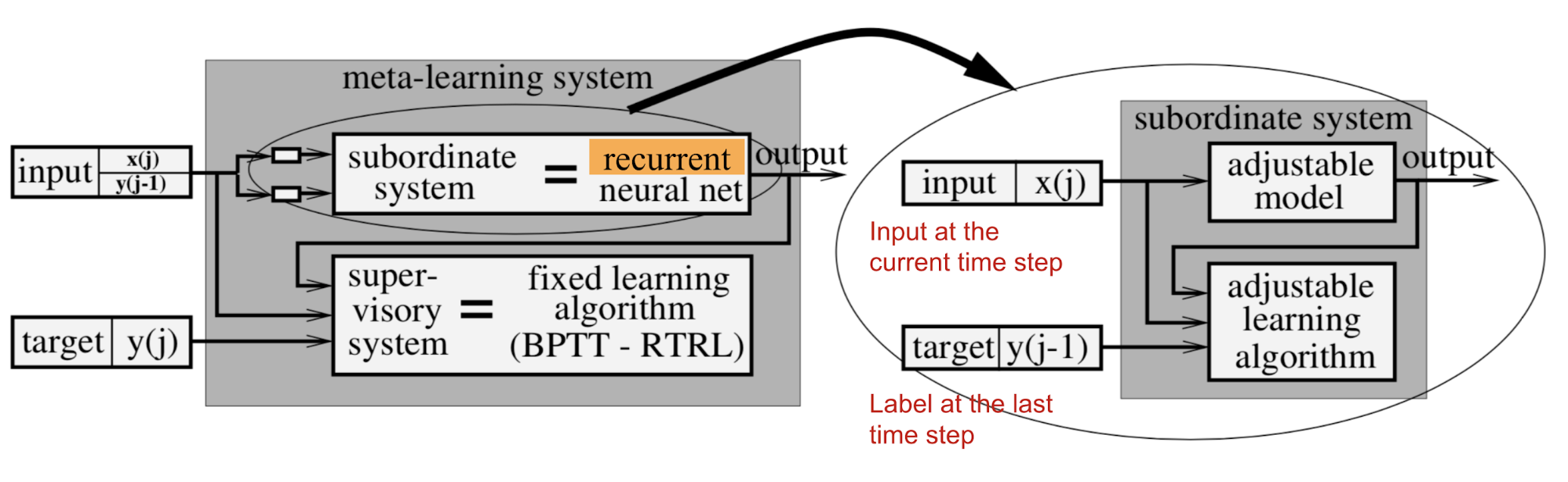
Hochreiter’s meta-learning model is a recurrent network with an LSTM cell. LSTM is a good choice because it can internalize a history of inputs and tune its own weights effectively through BPTT. The training data contains $K$ sequences, and each sequence consists of $N$ samples generated by a target function $f_k(.), k=1, \dots, K$,
Note that the last label $\mathbf{y}^k_{i-1}$ is also provided as an auxiliary input, enabling the function to learn the presented mapping.
In the experiment on decoding two-dimensional quadratic functions, $a x_1^2 + b x_2^2 + c x_1 x_2 + d x_1 + e x_2 + f$, with coefficients $a$-$f$ randomly sampled from [-1, 1], this meta-learning system was able to approximate the function after seeing only ~35 examples.
Proposal in 2016
In the modern era of DL, Wang et al. (2016) and Duan et al. (2017) proposed highly similar ideas simultaneously under the umbrella of Meta-RL (called RL^2 in the second paper). A meta-RL model is trained over a distribution of MDPs and, at test time, can learn to solve a new task quickly. Meta-RL sets an ambitious target by taking another step toward general algorithms.
Define Meta-RL
Meta Reinforcement Learning, in short, means doing meta-learning within the domain of reinforcement learning. Typically, the training and test tasks differ, but they are drawn from the same family of problems. For example, experiments in the papers included multi-armed bandits with different reward probabilities, mazes with different layouts, the same robots with different physical parameters in simulation, and many others.
Formulation
Assume we have a distribution of tasks, each formalized as an MDP (Markov Decision Process), $M_i \in \mathcal{M}$. An MDP is defined by a 4-tuple, $M_i= \langle \mathcal{S}, \mathcal{A}, P_i, R_i \rangle$:
| Symbol | Meaning |
|---|---|
| $\mathcal{S}$ | A set of states. |
| $\mathcal{A}$ | A set of actions. |
| $P_i: \mathcal{S} \times \mathcal{A} \times \mathcal{S} \to \mathbb{R}_{+}$ | Transition probability function. |
| $R_i: \mathcal{S} \times \mathcal{A} \to \mathbb{R}$ | Reward function. |
(The RL^2 paper adds an extra parameter, horizon $T$, to the MDP tuple to highlight that each MDP should have a finite horizon.)
Note that a shared state space $\mathcal{S}$ and action space $\mathcal{A}$ are used above, so that a (stochastic) policy: $\pi_\theta: \mathcal{S} \times \mathcal{A} \to \mathbb{R}_{+}$ receives inputs that are compatible across different tasks. The test tasks are sampled from the same distribution $\mathcal{M}$ or from a slightly modified version.
Main Differences from RL
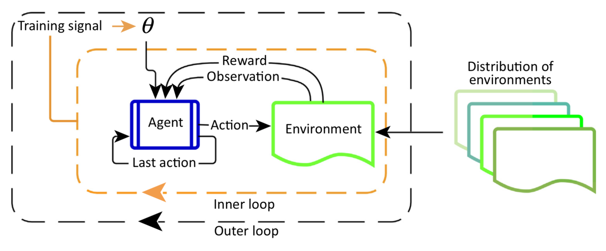
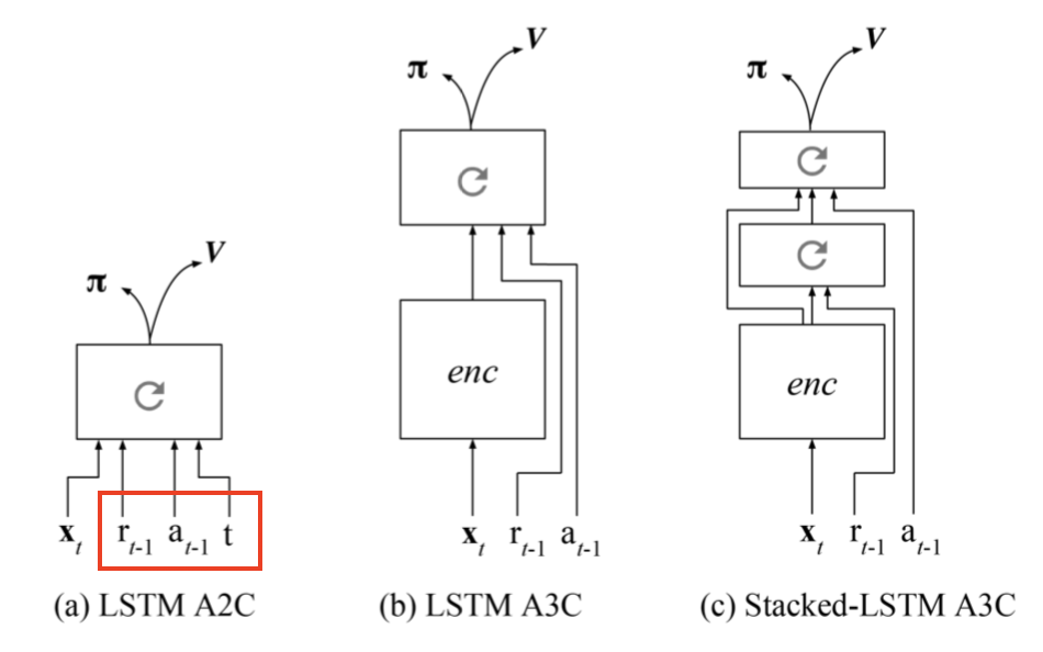
The overall configuration of meta-RL closely resembles an ordinary RL algorithm, except that the last reward $r_{t-1}$ and the last action $a_{t-1}$ are included in the policy observation in addition to the current state $s_t$.
- In RL: $\pi_\theta(s_t) \to$ a distribution over $\mathcal{A}$
- In meta-RL: $\pi_\theta(a_{t-1}, r_{t-1}, s_t) \to$ a distribution over $\mathcal{A}$
The motivation is to provide the model with a history so that the policy can internalize the relationships among states, rewards, and actions in the current MDP and adjust its strategy accordingly. This matches the setup in Hochreiter’s system. Both meta-RL and RL^2 implemented an LSTM policy, and the LSTM hidden states act as a memory that tracks characteristics of the trajectories. Because the policy is recurrent, there is no need to provide the last state explicitly as an input.
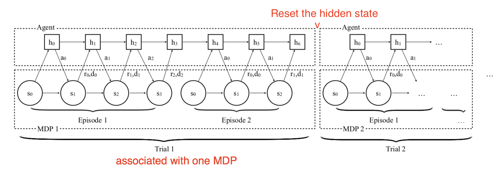
The training procedure is as follows:
- Sample a new MDP, $M_i \sim \mathcal{M}$;
- Reset the hidden state of the model;
- Collect multiple trajectories and update the model weights;
- Repeat from step 1.
Key Components
Meta-RL has three key components:
⭐ A Model with Memory
A recurrent neural network maintains a hidden state. As a result, it can acquire and store knowledge about the current task by updating that hidden state during rollouts. Without memory, meta-RL would not work.
⭐ Meta-learning Algorithm
A meta-learning algorithm specifies how to update model weights so that the model can solve an unseen task quickly at test time. In both the Meta-RL and RL^2 papers, the meta-learning algorithm is the standard gradient descent update of the LSTM, with the hidden state reset when switching between MDPs.
⭐ A Distribution of MDPs
Because the agent is exposed to a variety of environments and tasks during training, it must learn how to adapt across different MDPs.
According to Botvinick et al. (2019), one reason RL training can be slow is weak inductive bias ( = “a set of assumptions that the learner uses to predict outputs given inputs that it has not encountered”). As a general ML principle, a learning algorithm with weak inductive bias can cover a wider range of variation, but it is often less sample-efficient. Therefore, narrowing the hypothesis space with stronger inductive biases helps accelerate learning.
In meta-RL, we impose particular inductive biases from the task distribution and store them in memory. Which inductive bias is used at test time depends on the algorithm. Together, these three components provide a compelling perspective on meta-RL: adjusting the weights of a recurrent network is slow, but it enables the model to solve a new task quickly using its own RL algorithm implemented through internal activity dynamics.
Meta-RL also, interestingly and not unexpectedly, aligns with the ideas in the AI-GAs (“AI-Generating Algorithms”) paper by Jeff Clune (2019). He argued that one efficient path toward general AI is to make learning as automatic as possible. The AI-GAs approach is built on three pillars: (1) meta-learning architectures, (2) meta-learning algorithms, and (3) automatically generated environments for effective learning.
Designing strong recurrent network architectures is a broad topic and is outside the scope of this post, so I will skip it here. Next, we will examine the other two components more closely: meta-learning algorithms in the context of meta-RL, and methods for obtaining a diverse set of training MDPs.
Meta-Learning Algorithms for Meta-RL
My previous post on meta-learning covered several classic meta-learning algorithms. Here, I will include additional material that is more directly related to RL.
Optimizing Model Weights for Meta-learning
Both MAML (Finn, et al. 2017) and Reptile (Nichol et al., 2018) are methods for updating model parameters in order to achieve strong generalization performance on new tasks. See an earlier post section on MAML and Reptile.
Meta-learning Hyperparameters
The return function in an RL problem, $G_t^{(n)}$ or $G_t^\lambda$, includes several hyperparameters that are often chosen heuristically, such as the discount factor $\gamma$ and the bootstrapping parameter $\lambda$. Meta-gradient RL (Xu et al., 2018) treats them as meta-parameters, $\eta=\{\gamma, \lambda \}$, which can be tuned and learned online while an agent interacts with the environment. Therefore, the return becomes a function of $\eta$ and adapts dynamically to a specific task over time.
During training, we want to update the policy parameters using gradients as a function of all available information, $\theta’ = \theta + f(\tau, \theta, \eta)$, where $\theta$ are the current model weights, $\tau$ is a sequence of trajectories, and $\eta$ are the meta-parameters.
Meanwhile, assume we have a meta-objective function $J(\tau, \theta, \eta)$ as a performance measure. The training process follows the idea of online cross-validation, using a sequence of consecutive experiences:
- Starting with parameter $\theta$, the policy $\pi_\theta$ is updated on the first batch of samples $\tau$, resulting in $\theta’$.
- Next, we continue running the policy $\pi_{\theta’}$ to collect a new set of experiences $\tau’$, proceeding consecutively in time after $\tau$. Performance is measured as $J(\tau’, \theta’, \bar{\eta})$ with a fixed meta-parameter $\bar{\eta}$.
- The gradient of the meta-objective $J(\tau’, \theta’, \bar{\eta})$ w.r.t. $\eta$ is then used to update $\eta$:
where $\beta$ is the learning rate for $\eta$.
The meta-gradient RL algorithm simplifies computation by setting the secondary gradient term to zero, $\mathbf{I} + \partial g(\tau, \theta, \eta)/\partial\theta = 0$. This choice prioritizes the immediate effect of the meta-parameters $\eta$ on the parameters $\theta$. We then obtain:
Experiments in the paper used the same type of meta-objective function as the $TD(\lambda)$ algorithm, minimizing the error between the approximated value function $v_\theta(s)$ and the $\lambda$-return:
Meta-learning the Loss Function
In policy gradient algorithms, the expected total reward is maximized by updating the policy parameters $\theta$ in the direction of the estimated gradient (Schulman et al., 2016),
where common candidates for $\Psi_t$ include the trajectory return $G_t$, the Q value $Q(s_t, a_t)$, or the advantage value $A(s_t, a_t)$. The corresponding surrogate loss function for policy gradients can be reverse-engineered as:
This loss function is defined over a history of trajectories, $(s_0, a_0, r_0, \dots, s_t, a_t, r_t, \dots)$. Evolved Policy Gradient (EPG; Houthooft, et al, 2018) goes further by defining the policy gradient loss function as a temporal convolution (1-D convolution) over the agent’s past experience, $L_\phi$. The parameters $\phi$ of the loss-function network are evolved so that an agent can achieve higher returns.
As with many meta-learning algorithms, EPG uses two optimization loops:
- In the inner loop, an agent learns to improve its policy $\pi_\theta$.
- In the outer loop, the model updates the parameters $\phi$ of the loss function $L_\phi$. Because there is no explicit way to express a differentiable equation linking return and loss, EPG relies on Evolutionary Strategies (ES).
The general approach is to train a population of $N$ agents. Each agent is trained using the loss function $L_{\phi + \sigma \epsilon_i}$ parameterized by $\phi$, with small Gaussian noise $\epsilon_i \sim \mathcal{N}(0, \mathbf{I})$ of standard deviation $\sigma$ added. During inner-loop training, EPG maintains a history of experience and updates the policy parameters using the loss function $L_{\phi + \sigma\epsilon_i}$ for each agent:
where $\alpha_\text{in}$ is the inner-loop learning rate, and $\tau_{t-K, \dots, t}$ is a sequence of $M$ transitions up to the current time step $t$.
Once the inner-loop policy is sufficiently mature, it is evaluated using the mean return $\bar{G}_{\phi+\sigma\epsilon_i}$ over multiple randomly sampled trajectories. Eventually, we can estimate the gradient of $\phi$ numerically according to NES (Salimans et al, 2017). As this process repeats, both the policy parameters $\theta$ and the loss-function weights $\phi$ are updated simultaneously to increase returns.
where $\alpha_\text{out}$ is the learning rate of the outer loop.
In practice, the loss $L_\phi$ is bootstrapped using an ordinary policy gradient surrogate loss $L_\text{pg}$, $\hat{L} = (1-\alpha) L_\phi + \alpha L_\text{pg}$ (such as REINFORCE or PPO). The weight $\alpha$ is annealed gradually from 1 to 0 during training. At test time, the loss-function parameter $\phi$ remains fixed, and the loss value is computed over a history of experience to update the policy parameters $\theta$.
Meta-learning the Exploration Strategies
The exploitation vs exploration dilemma is a fundamental challenge in RL. Common exploration strategies include $\epsilon$-greedy, adding random noise to actions, or using a stochastic policy with built-in randomness in the action space.
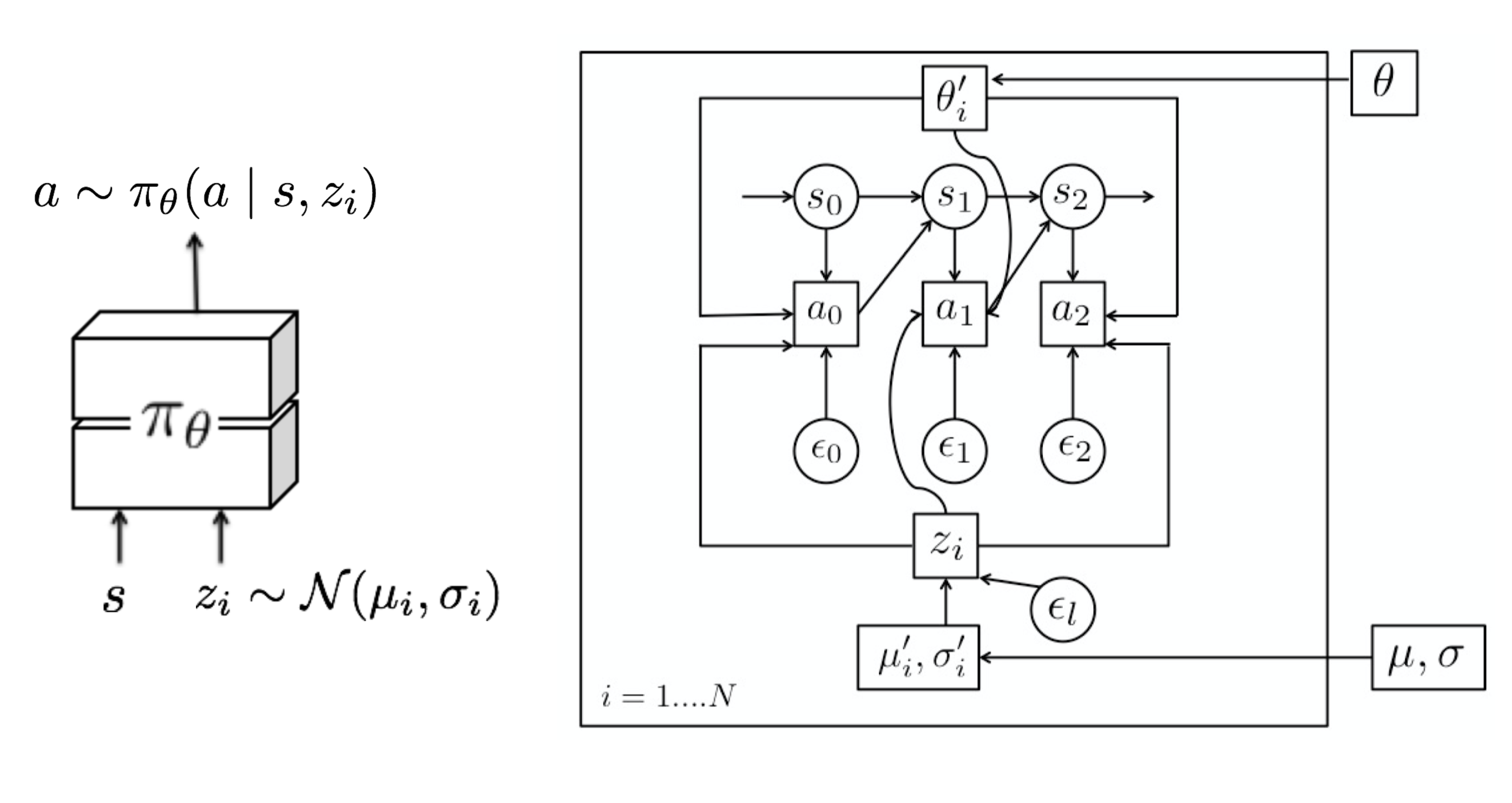
MAESN (Gupta et al, 2018) is an algorithm that learns structured action noise from prior experience to enable better and more effective exploration. Simply injecting random noise into actions does not capture task-dependent or time-correlated exploration strategies. MAESN modifies the policy to condition on a per-task random variable $z_i \sim \mathcal{N}(\mu_i, \sigma_i)$; for the $i$-th task $M_i$, we obtain a policy $a \sim \pi_\theta(a\mid s, z_i)$. The latent variable $z_i$ is sampled once and held fixed for one episode. Intuitively, the latent variable selects a type of behavior (or skill) to explore more heavily at the start of a rollout, and the agent adjusts its actions accordingly. Both the policy parameters and the latent space are optimized to maximize total task rewards. At the same time, the policy learns to leverage the latent variables for exploration.
In addition, the loss function includes a KL divergence between the learned latent variable and a unit Gaussian prior, $D_\text{KL}(\mathcal{N}(\mu_i, \sigma_i)|\mathcal{N}(0, \mathbf{I}))$. On the one hand, this constrains the learned latent space so it does not drift too far from a shared prior. On the other hand, it forms the variational evidence lower bound (ELBO) for the reward function. Interestingly, the paper found that $(\mu_i, \sigma_i)$ for each task are usually close to the prior at convergence.
Episodic Control
A major criticism of RL concerns sample inefficiency. RL often requires many samples and small learning steps for incremental parameter updates, both to maximize generalization and to avoid catastrophic forgetting of earlier learning (Botvinick et al., 2019).
Episodic control (Lengyel & Dayan, 2008) is proposed as a way to reduce forgetting and improve generalization while enabling faster training. It is partially inspired by hypotheses about instance-based hippocampal learning.
An episodic memory stores explicit records of past events and uses those records directly as reference points for new decisions (that is, similar to metric-based meta-learning). In MFEC (Model-Free Episodic Control; Blundell et al., 2016), memory is represented as a large table that uses the state-action pair $(s, a)$ as the key and stores the corresponding Q-value $Q_\text{EC}(s, a)$ as the value. When a new observation $s$ is received, the Q value is estimated non-parametrically as the average Q-value of the top $k$ most similar samples:
where $s^{(i)}, i=1, \dots, k$ are the top $k$ states with the smallest distances to the state $s$. The action that yields the highest estimated Q value is then selected. The memory table is updated according to the return received at $s_t$:
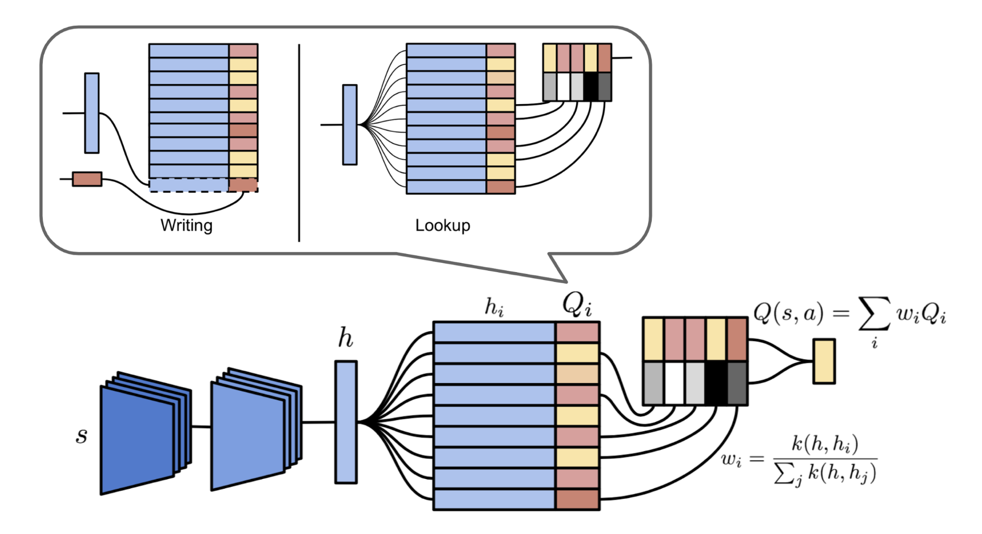
As a tabular RL method, MFEC suffers from high memory usage and limited ability to generalize across similar states. The first issue can be addressed with an LRU cache. Inspired by metric-based meta-learning, especially Matching Networks (Vinyals et al., 2016), the generalization issue is improved in a follow-up algorithm, NEC (Neural Episodic Control; Pritzel et al., 2016).
In NEC, episodic memory is implemented as a Differentiable Neural Dictionary (DND). The key is a convolutional embedding vector derived from input image pixels, and the value stores the estimated Q value. Given a query key, the output is a weighted sum of the values associated with the most similar keys, where weights are computed as a normalized kernel measure between the query key and each selected key in the dictionary. This resembles a hard attention machanism.
In addition, Episodic LSTM (Ritter et al., 2018) augments the standard LSTM architecture with a DND-based episodic memory that stores task-context embeddings as keys and LSTM cell states as values. The model retrieves the saved hidden states and adds them directly to the current cell state using the same gating mechanism already present in the LSTM:
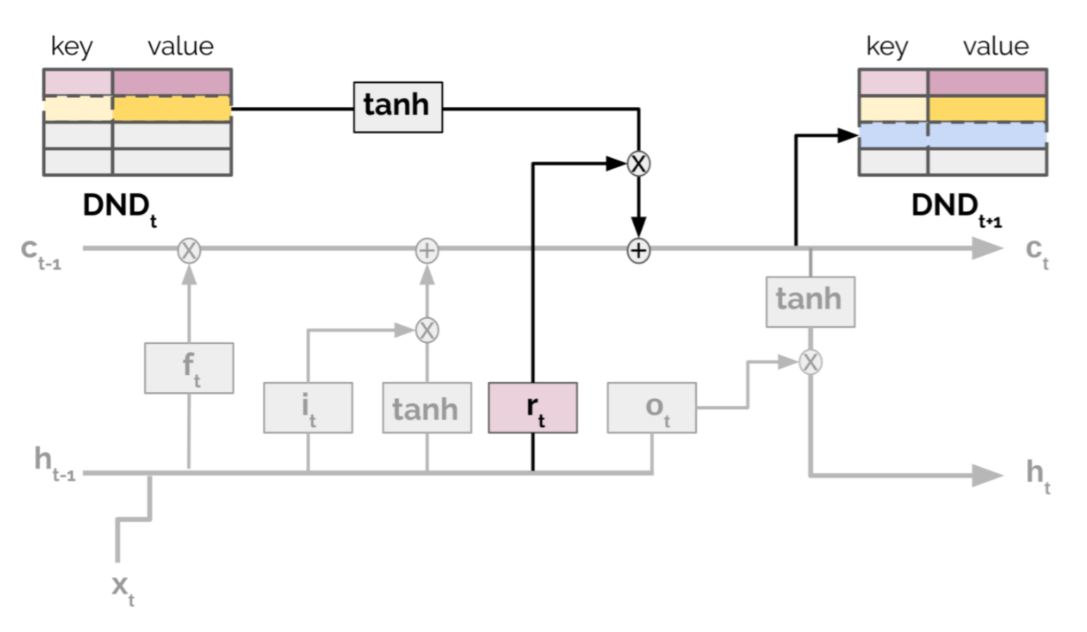
Here, $\mathbf{c}_t$ and $\mathbf{h}_t$ denote the hidden state and cell state at time $t$. $\mathbf{i}_t$, $\mathbf{f}_t$, and $\mathbf{r}_t$ are the input, forget, and reinstatement gates, respectively. $\mathbf{c}_\text{ep}$ is the cell state retrieved from episodic memory. The newly introduced episodic-memory components are highlighted in green.
This design creates a shortcut to prior experience via context-conditioned retrieval. At the same time, explicitly storing task-dependent experience in external memory helps prevent forgetting. In the paper, all experiments rely on manually constructed context vectors. How to build an effective and efficient representation for task-context embeddings in more free-form tasks remains an interesting direction.
More broadly, the capacity of episodic control is constrained by environmental complexity. In real-world tasks, it is uncommon for an agent to revisit exactly the same states repeatedly, so accurate state encoding becomes critical. A learned embedding space compresses observations into a lower-dimensional representation and, concurrently, states that are nearby in this space are expected to require similar strategies.
Training Task Acquisition
Of the three key components, designing an appropriate task distribution is the least explored and is arguably the aspect most specific to meta-RL itself. As described above, each task is an MDP: $M_i = \langle \mathcal{S}, \mathcal{A}, P_i, R_i \rangle \in \mathcal{M}$. A distribution over MDPs can be constructed by varying the following:
- The reward configuration: Across tasks, the same behavior may be rewarded differently according to $R_i$.
- Or, the environment: The transition function $P_i$ can be altered by initializing the environment with different shifts between states.
Task Generation by Domain Randomization
Randomizing simulator parameters is a straightforward way to create tasks with modified transition functions. If you would like to study this topic further, see my previous post on domain randomization.
Evolutionary Algorithm on Environment Generation
Evolutionary algorithm is a gradient-free, heuristic optimization approach inspired by natural selection. It maintains a population of candidate solutions and iterates through evaluation, selection, reproduction, and mutation. Over time, stronger solutions persist and are preferentially selected.
POET (Wang et al, 2019), an evolutionary-algorithm-based framework, aims to generate tasks while simultaneously solving them. Although the POET implementation is tailored specifically to a simple 2D bipedal walker environment, it highlights an intriguing research direction. It is also worth noting that evolutionary algorithms have produced compelling results in deep learning, including EPG and PBT (Population-Based Training; Jaderberg et al, 2017).
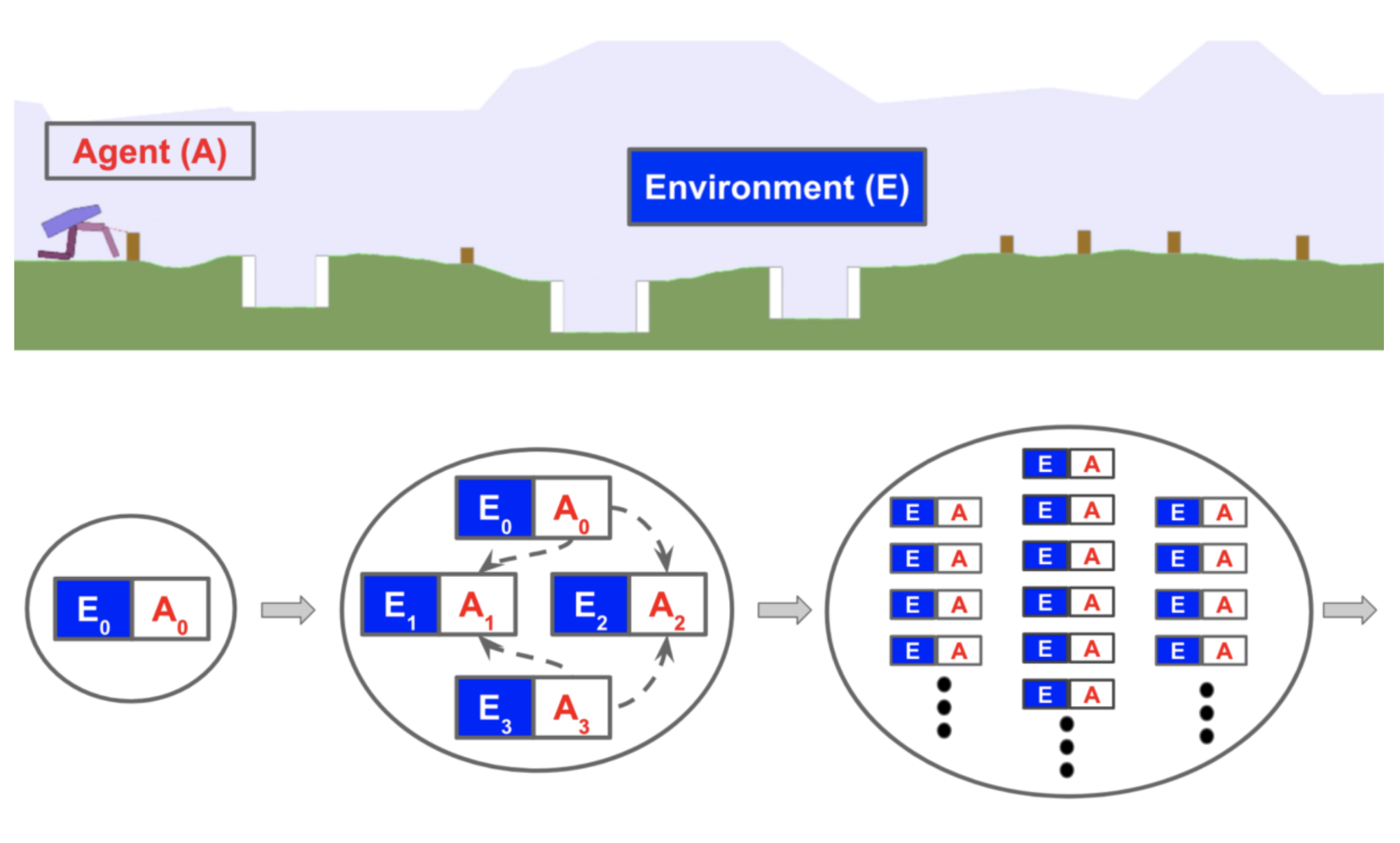
In POET, the 2D bipedal walking environment evolves from a simple flat surface into substantially more challenging trails that may include gaps, stumps, and rough terrain. POET couples the creation of environmental challenges with agent optimization in order to (a) select agents capable of solving the current challenges and (b) evolve environments so they remain solvable. The algorithm maintains a set of environment-agent pairs and repeatedly performs the following steps:
- Mutation: Create new environments from currently active environments. Note that the mutation operators here are designed specifically for the bipedal walker, and a different environment would require a different configuration set.
- Optimization: Train each paired agent in its corresponding environment.
- Selection: Periodically attempt to transfer agents between environments. For each environment, copy and update the best-performing agent. The underlying intuition is that competencies learned in one environment may transfer to another.
This procedure closely resembles PBT, except that PBT mutates and evolves hyperparameters instead. In a sense, POET is performing domain randomization, since gaps, stumps, and terrain roughness are governed by randomized probability parameters. Unlike DR, agents are not exposed to a fully randomized difficult environment all at once. Instead, they learn progressively through a curriculum shaped by the evolutionary algorithm.
Learning with Random Rewards
An MDP without a reward function $R$ is referred to as a Controlled Markov process (CMP). Given a predefined CMP, $\langle \mathcal{S}, \mathcal{A}, P\rangle$, we can obtain a range of tasks by generating a set of reward functions $\mathcal{R}$ that promote learning an effective meta-learning policy.
Gupta et al. (2018) introduced two unsupervised methods for expanding the task distribution in the CMP setting. Assuming an underlying latent variable $z \sim p(z)$ for each task, this variable parameterizes (or determines) a reward function: $r_z(s) = \log D(z|s)$. A “discriminator” function $D(.)$ is used to infer the latent variable from the state. The paper outlines two approaches for defining the discriminator function:
- Sample random discriminator weights $\phi_\text{rand}$, $D_{\phi_\text{rand}}(z \mid s)$.
- Learn a discriminator function that encourages diversity-driven exploration. This approach is described in more detail in a related paper, “DIAYN” (Eysenbach et al., 2018).
DIAYN, short for “Diversity is all you need”, is a framework that encourages a policy to acquire useful skills without relying on a reward function. It explicitly treats the latent variable $z$ as a skill embedding and conditions the policy on $z$ in addition to the state $s$, $\pi_\theta(a \mid s, z)$. (This section is the same as MAESN, unsurprisingly, since both papers come from the same group.) The DIAYN design is motivated by several hypotheses:
- Skills should be diverse and should drive visitation of different states. → maximize the mutual information between states and skills, $I(S; Z)$
- Skills should be distinguishable from states rather than actions. → minimize the mutual information between actions and skills, conditioned on states $I(A; Z \mid S)$
The maximization objective is given below, where policy entropy is included as well to promote diversity:
In this expression, $I(.)$ denotes mutual information, and $H[.]$ is an entropy measure. Because we cannot integrate over all states to compute $p(z \mid s)$, we instead approximate it with $D_\phi(z \mid s)$, namely, the diversity-driven discriminator function.
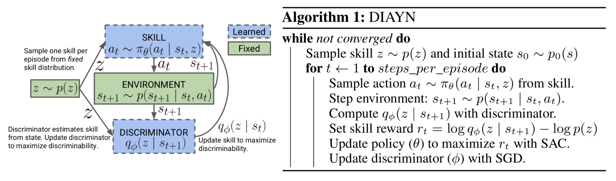
After learning the discriminator function, sampling a new MDP for training becomes straightforward. First, sample a latent variable $z \sim p(z)$ and construct a reward function $r_z(s) = \log(D(z \vert s))$. Combining this reward function with the predefined CMP yields a new MDP.
--- So far, experiments of meta-RL are still limited to a collection of very similar tasks, originated from the same family; such as multi-armed bandit with different reward probabilities, mazes with different layouts, or same robots but with different physical parameters in simulator. I'm looking forward to more research demonstrating the power of meta-RL over a more diverse set of tasks.Cited as:
@article{weng2019metaRL,
  title   = "Meta Reinforcement Learning",
  author  = "Weng, Lilian",
  journal = "lilianweng.github.io",
  year    = "2019",
  url     = "https://lilianweng.github.io/posts/2019-06-23-meta-rl/"
}
References
[1] Richard S. Sutton. “The Bitter Lesson.” March 13, 2019.
[2] Sepp Hochreiter, A. Steven Younger, and Peter R. Conwell. “Learning to learn using gradient descent.” Intl. Conf. on Artificial Neural Networks. 2001.
[3] Jane X Wang, et al. “Learning to reinforcement learn.” arXiv preprint arXiv:1611.05763 (2016).
[4] Yan Duan, et al. “RL $^ 2$: Fast Reinforcement Learning via Slow Reinforcement Learning.” ICLR 2017.
[5] Matthew Botvinick, et al. “Reinforcement Learning, Fast and Slow” Cell Review, Volume 23, Issue 5, P408-422, May 01, 2019.
[6] Jeff Clune. “AI-GAs: AI-generating algorithms, an alternate paradigm for producing general artificial intelligence” arXiv preprint arXiv:1905.10985 (2019).
[7] Zhongwen Xu, et al. “Meta-Gradient Reinforcement Learning” NIPS 2018.
[8] Rein Houthooft, et al. “Evolved Policy Gradients.” NIPS 2018.
[9] Tim Salimans, et al. “Evolution strategies as a scalable alternative to reinforcement learning.” arXiv preprint arXiv:1703.03864 (2017).
[10] Abhishek Gupta, et al. “Meta-Reinforcement Learning of Structured Exploration Strategies.” NIPS 2018.
[11] Alexander Pritzel, et al. “Neural episodic control.” Proc. Intl. Conf. on Machine Learning, Volume 70, 2017.
[12] Charles Blundell, et al. “Model-free episodic control.” arXiv preprint arXiv:1606.04460 (2016).
[13] Samuel Ritter, et al. “Been there, done that: Meta-learning with episodic recall.” ICML, 2018.
[14] Rui Wang et al. “Paired Open-Ended Trailblazer (POET): Endlessly Generating Increasingly Complex and Diverse Learning Environments and Their Solutions” arXiv preprint arXiv:1901.01753 (2019).
[15] Uber Engineering Blog: “POET: Endlessly Generating Increasingly Complex and Diverse Learning Environments and their Solutions through the Paired Open-Ended Trailblazer.” Jan 8, 2019.
[16] Abhishek Gupta, et al.“Unsupervised meta-learning for Reinforcement Learning” arXiv preprint arXiv:1806.04640 (2018).
[17] Eysenbach, Benjamin, et al. “Diversity is all you need: Learning skills without a reward function.” ICLR 2019.
[18] Max Jaderberg, et al. “Population Based Training of Neural Networks.” arXiv preprint arXiv:1711.09846 (2017).