Evolution Strategies
Stochastic gradient descent is a widely used default for optimizing deep learning models, but it is not the only viable approach. Black-box optimization algorithms allow you to evaluate a target function $f(x): \mathbb{R}^n \to \mathbb{R}$ even when you do not know the exact analytic form of $f(x)$ and therefore cannot compute gradients or the Hessian matrix. Representative black-box optimization methods include Simulated Annealing, Hill Climbing, and the Nelder-Mead method.
· 22 min read · Curated and presented by Arthur Sedek
Stochastic gradient descent is a widely used method for optimizing deep learning models, but it is not the only option. With black-box optimization algorithms, you can evaluate a target function $f(x): \mathbb{R}^n \to \mathbb{R}$ even when you do not know the precise analytic form of $f(x)$, and therefore cannot compute gradients or the Hessian matrix. Examples of black-box optimization methods include Simulated Annealing, Hill Climbing, and the Nelder-Mead method.
Evolution Strategies (ES) are one class of black-box optimization algorithms, originating within the broader family of Evolutionary Algorithms (EA). In this post, I will examine a few classic ES methods and introduce several ways ES can contribute to deep reinforcement learning.
What are Evolution Strategies?
Evolution strategies (ES) belong to the larger family of evolutionary algorithms. ES typically optimize vectors of real numbers, $x \in \mathbb{R}^n$.
Evolutionary algorithms are a category of population-based optimization methods inspired by natural selection. Natural selection holds that individuals with traits that improve survival are more likely to persist across generations and to pass on favorable characteristics. Over time, selection drives evolutionary change, and the population becomes increasingly well adapted to its environment.
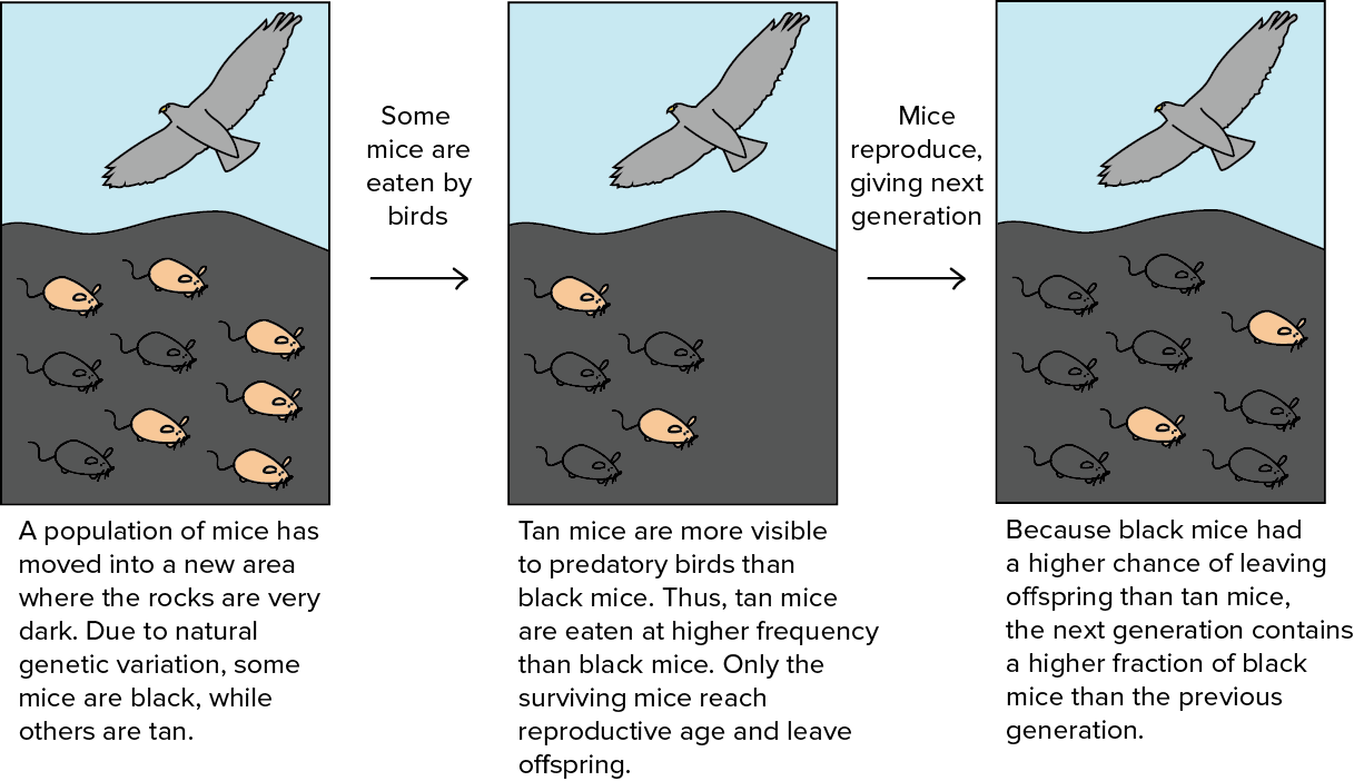
Evolutionary algorithms can be expressed in the following format as a general-purpose optimization procedure:
Suppose we aim to optimize a function $f(x)$ and cannot compute gradients directly. However, we can still evaluate $f(x)$ for any $x$, and the result is deterministic. Our belief over $x$ as a good solution to the $f(x)$ optimization problem is represented by $p_\theta(x)$, parameterized by $\theta$. The objective is to identify an optimal configuration of $\theta$.
Given a fixed distribution family (for example, Gaussian), the parameter $\theta$ encodes knowledge about the best solutions and is updated iteratively across generations.
Starting from an initial value $\theta$, we repeatedly update $\theta$ by cycling through the following three steps:
- Generate a population of samples $D = \{(x_i, f(x_i)\}$ where $x_i \sim p_\theta(x)$.
- Evaluate the “fitness” of the samples in $D$.
- Select the best subset of individuals and use them to update $\theta$, typically based on fitness or rank.
In Genetic Algorithms (GA), another widely used EA subcategory, $x$ is represented as a sequence of binary codes, $x \in \{0, 1\}^n$. In contrast, ES uses $x$ as a vector of real numbers, $x \in \mathbb{R}^n$.
Simple Gaussian Evolution Strategies
This is the most basic and canonical form of evolution strategies. It models $p_\theta(x)$ as a $n$-dimensional isotropic Gaussian distribution, where $\theta$ tracks only the mean $\mu$ and the standard deviation $\sigma$.
The Simple-Gaussian-ES procedure, given $x \in \mathcal{R}^n$, is as follows:
- Initialize $\theta = \theta^{(0)}$ and the generation counter $t=0$.
- Generate an offspring population of size $\Lambda$ by sampling from the Gaussian distribution:
$D^{(t+1)}=\{ x^{(t+1)}_i \mid x^{(t+1)}_i = \mu^{(t)} + \sigma^{(t)} y^{(t+1)}_i \text{ where } y^{(t+1)}_i \sim \mathcal{N}(x \vert 0, \mathbf{I}),;i = 1, \dots, \Lambda\}$
. - Select a top subset of $\lambda$ samples with optimal $f(x_i)$. This subset is referred to as the elite set. Without loss of generality, we can treat the first $k$ samples in $D^{(t+1)}$ as belonging to the elite group, and label them as follows:
- Estimate the mean and standard deviation for the next generation using the elite set:
- Repeat steps (2) through (4) until the result is good enough ✌️
Covariance Matrix Adaptation Evolution Strategies (CMA-ES)
The standard deviation $\sigma$ determines the amount of exploration: the larger $\sigma$ is, the larger the region from which we can sample the offspring population. In vanilla ES, $\sigma^{(t+1)}$ is strongly correlated with $\sigma^{(t)}$, which prevents the algorithm from quickly adapting the exploration scale when necessary (for example, when the confidence level changes).
CMA-ES, short for “Covariance Matrix Adaptation Evolution Strategy”, addresses this limitation by tracking pairwise dependencies among samples in the distribution using a covariance matrix $C$. The updated distribution parameters become:
where $\sigma$ controls the overall scale of the distribution and is often referred to as the step size.
Before describing how CMA-ES updates these parameters, it is helpful to review the role of the covariance matrix in a multivariate Gaussian distribution. As a real symmetric matrix, the covariance matrix $C$ has several useful properties (see proof and proof):
- It is always diagonalizable.
- It is always positive semi-definite.
- All eigenvalues are real and non-negative.
- All eigenvectors are orthogonal.
- There exists an orthonormal basis of $\mathbb{R}^n$ consisting of its eigenvectors.
Let the matrix $C$ have an orthonormal eigenvector basis $B = [b_1, \dots, b_n]$ with corresponding eigenvalues $\lambda_1^2, \dots, \lambda_n^2$. Let $D=\text{diag}(\lambda_1, \dots, \lambda_n)$.
The square root of $C$ is:
| Symbol | Meaning |
|---|---|
| $x_i^{(t)} \in \mathbb{R}^n$ | the $i$-th samples at the generation (t) |
| $y_i^{(t)} \in \mathbb{R}^n$ | $x_i^{(t)} = \mu^{(t-1)} + \sigma^{(t-1)} y_i^{(t)} $ |
| $\mu^{(t)}$ | mean of the generation (t) |
| $\sigma^{(t)}$ | step size |
| $C^{(t)}$ | covariance matrix |
| $B^{(t)}$ | a matrix of $C$’s eigenvectors as row vectors |
| $D^{(t)}$ | a diagonal matrix with $C$’s eigenvalues on the diagnose. |
| $p_\sigma^{(t)}$ | evaluation path for $\sigma$ at the generation (t) |
| $p_c^{(t)}$ | evaluation path for $C$ at the generation (t) |
| $\alpha_\mu$ | learning rate for $\mu$’s update |
| $\alpha_\sigma$ | learning rate for $p_\sigma$ |
| $d_\sigma$ | damping factor for $\sigma$’s update |
| $\alpha_{cp}$ | learning rate for $p_c$ |
| $\alpha_{c\lambda}$ | learning rate for $C$’s rank-min(λ, n) update |
| $\alpha_{c1}$ | learning rate for $C$’s rank-1 update |
Updating the Mean
CMA-ES uses a learning rate $\alpha_\mu \leq 1$ to control how quickly the mean $\mu$ is updated. It is commonly set to 1, in which case the equation matches vanilla ES, $\mu^{(t+1)} = \frac{1}{\lambda}\sum_{i=1}^\lambda (x_i^{(t+1)}$.
Controlling the Step Size
The sampling procedure can be separated from the mean and standard deviation:
The parameter $\sigma$ governs the overall scale of the distribution. It is factored out of the covariance matrix so that the step size can be adjusted more rapidly than the full covariance. A larger step size produces faster parameter updates. To assess whether the current step size is appropriate, CMA-ES constructs an evolution path $p_\sigma$ by summing a consecutive sequence of movement steps, $\frac{1}{\lambda}\sum_{i}^\lambda y_i^{(j)}, j=1, \dots, t$. By comparing the resulting path length to its expected length under random selection (that is, when individual steps are uncorrelated), we can adjust $\sigma$ accordingly (see Fig. 2).
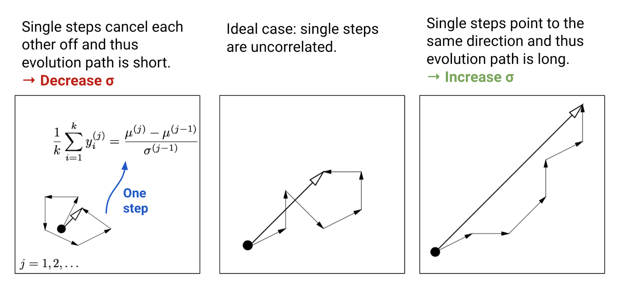
Each time, the evolution path is updated using the average movement step $y_i$ for the current generation.
By multiplying by $C^{-\frac{1}{2}}$, the evolution path is transformed to be independent of direction. The term ${C^{(t)}}^{-\frac{1}{2}} = {B^{(t)}}^\top {D^{(t)}}^{-\frac{1}{2}} {B^{(t)}}$ transformation works as follows:
- ${B^{(t)}}$ contains row vectors of $C$’s eigenvectors. It projects the original space onto perpendicular principal axes.
- ${D^{(t)}}^{-\frac{1}{2}} = \text{diag}(\frac{1}{\lambda_1}, \dots, \frac{1}{\lambda_n})$ then scales the principal-axis lengths so that they become equal.
- ${B^{(t)}}^\top$ transforms the space back into the original coordinate system.
To weight recent generations more heavily, we apply Polyak averaging to update the evolution path using learning rate $\alpha_\sigma$. At the same time, the weights are balanced so that $p_\sigma$ is conjugate, $\sim \mathcal{N}(0, I)$ both before and after one update.
The expected length of $p_\sigma$ under random selection is $\mathbb{E}|\mathcal{N}(0,I)|$, namely the expectation of the L2 norm of a $\mathcal{N}(0,I)$ random variable. Following the intuition in Fig. 2, we adjust the step size based on the ratio $|p_\sigma^{(t+1)}| / \mathbb{E}|\mathcal{N}(0,I)|$:
where $d_\sigma \approx 1$ is a damping parameter that scales how quickly $\ln\sigma$ is adjusted.
Adapting the Covariance Matrix
For the covariance matrix, one option is to estimate it from scratch using $y_i$ elite samples (recall that $y_i \sim \mathcal{N}(0, C)$):
This estimator is reliable only when the selected population is sufficiently large. However, we generally want fast iterations with a small population size per generation. For this reason, CMA-ES introduced a more robust, but also more complex, method for updating $C$. It uses two independent update routes:
- Rank-min(λ, n) update: uses the history of $\{C_\lambda\}$, each computed from scratch within a single generation.
- Rank-one update: estimates the movement steps $y_i$ and preserves sign information from the history.
The first route treats $C$ as an estimator derived from the full history of $\{C_\lambda\}$. For example, after many generations, $C^{(t+1)} \approx \text{avg}(C_\lambda^{(i)}; i=1,\dots,t)$ would serve as a strong estimator. As with $p_\sigma$, Polyak averaging is used with a learning rate to incorporate historical information:
A typical choice for the learning rate is $\alpha_{c\lambda} \approx \min(1, \lambda/n^2)$.
The second route addresses the fact that $y_i{y_i}^\top = (-y_i)(-y_i)^\top$ discards sign information. Analogous to step-size control $\sigma$, an evolution path $p_c$ is used to track sign information, and it is constructed so that $p_c$ is conjugate, $\sim \mathcal{N}(0, C)$ both before and after incorporating a new generation.
We can view $p_c$ as an alternative way to compute $\text{avg}_i(y_i)$ (noting that both $\sim \mathcal{N}(0, C)$), while leveraging the entire history and preserving sign information. Note that $\sqrt{k}\frac{\mu^{(t+1)} - \mu^{(t)}}{\sigma^{(t)}} \sim \mathcal{N}(0, C)$ was defined in the previous section:
The covariance matrix is then updated according to $p_c$:
The rank-one update method is claimed to yield a substantial improvement over the rank-min(λ, n)-update when $k$ is small, because it exploits the signs of movement steps and the correlations between consecutive steps, propagating both across generations.
Finally, the two approaches are combined:
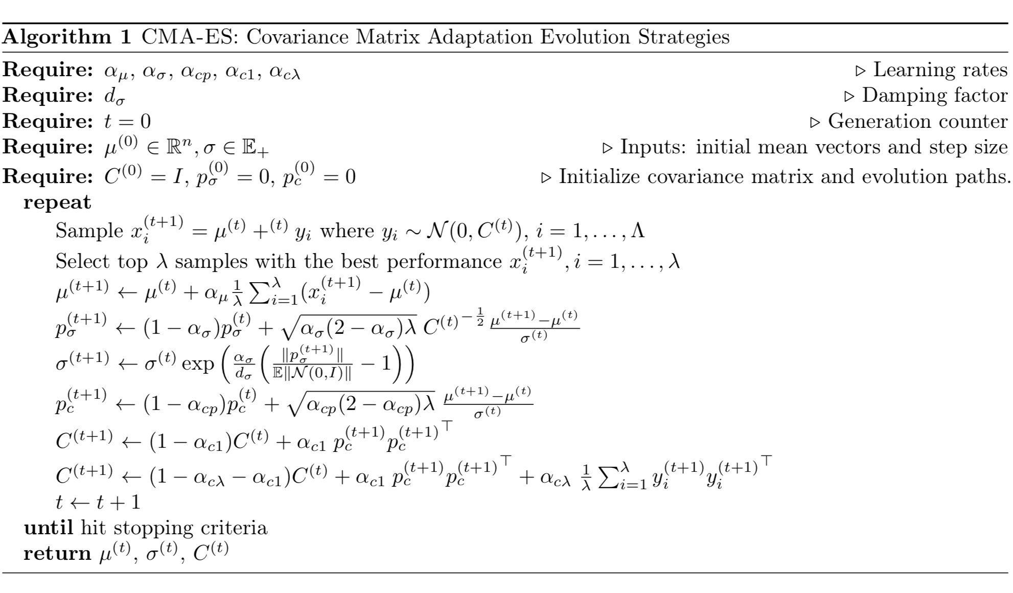
Across all of the examples above, each elite sample is assumed to contribute an equal amount of weight, $1/\lambda$. This procedure can be extended straightforwardly to the setting in which selected samples receive different weights, $w_1, \dots, w_\lambda$, based on their performance. For additional details, see the tutorial.
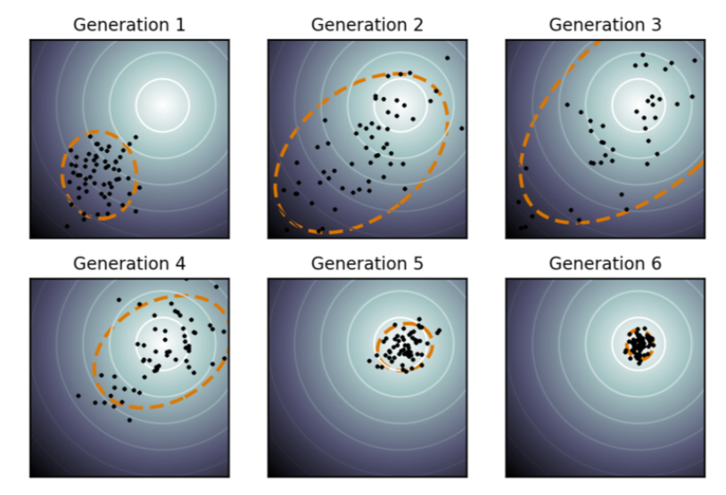
Natural Evolution Strategies
Natural Evolution Strategies (NES; Wierstra, et al, 2008) performs optimization over a search distribution of parameters, updating that distribution in the direction of higher fitness as indicated by the natural gradient.
Natural Gradients
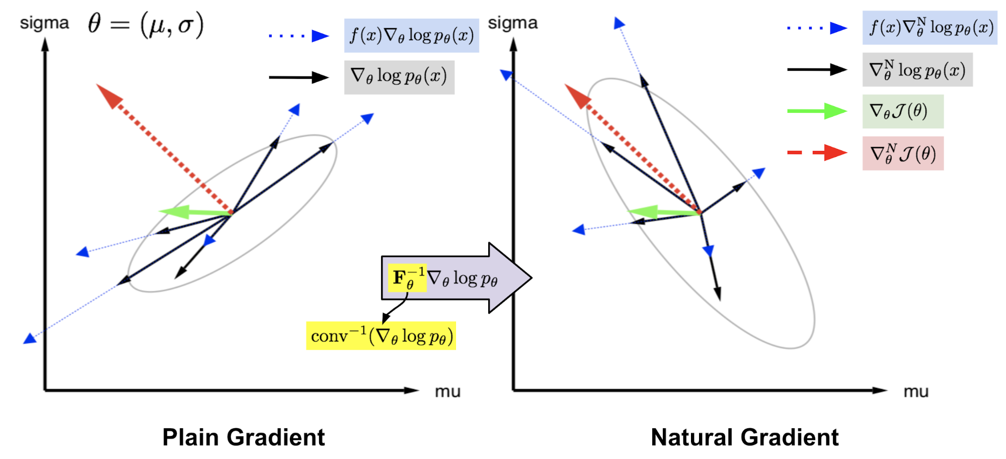
Given an objective function $\mathcal{J}(\theta)$ parameterized by $\theta$, suppose our goal is to find the optimal $\theta$ that maximizes the objective value. A plain gradient identifies the steepest direction subject to a small Euclidean distance from the current $\theta$. Here, the distance constraint is imposed in parameter space. Equivalently, we compute the plain gradient with respect to a small change in the absolute value of $\theta$. The optimal step is:
In contrast, the natural gradient operates in a probability distribution space parameterized by $\theta$, $p_\theta(x)$ (called the “search distribution” in the NES paper). It seeks the steepest direction under a small step in distribution space, where distance is measured using KL divergence. This constraint ensures that each update moves along the distributional manifold at a constant speed, rather than being slowed by curvature.
Estimation using Fisher Information Matrix
However, how do we compute $\text{KL}[p_\theta | p_{\theta+\Delta\theta}]$ exactly? By taking a Taylor expansion of $\log p_{\theta + d}$ around $\theta$, we obtain:
where
Therefore, we ultimately have:
where $\mathbf{F}_\theta$ is known as the Fisher Information Matrix, and it is the covariance matrix of $\nabla_\theta \log p_\theta$ because $\mathbb{E}[\nabla_\theta \log p_\theta] = 0$.
The solution to the following optimization problem:
can be derived using a Lagrangian multiplier:
where $d_\text{N}^*$ extracts only the direction of the optimal update step on $\theta$, while ignoring the scalar $\beta^{-1}$.
NES Algorithm
The fitness associated with one sample is denoted $f(x)$, and the search distribution over $x$ is parameterized by $\theta$. NES aims to optimize the parameter $\theta$ in order to maximize the expected fitness:
Applying the same log-likelihood trick used in REINFORCE:
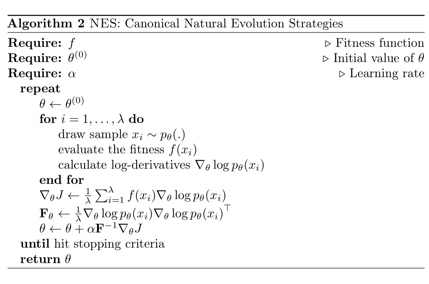
In addition to natural gradients, NES incorporates several key heuristics that improve robustness in practice.
- NES uses rank-based fitness shaping; that is, it uses the rank under monotonically increasing fitness values rather than $f(x)$ directly. Alternatively, it can use a function of the rank (a “utility function”), which NES treats as a free parameter.
- NES employs adaptation sampling to adjust hyperparameters at run time. When modifying $\theta \to \theta’$, samples drawn from $p_\theta$ are compared with samples from $p_{\theta’}$ using [Mann-Whitney U-test(https://en.wikipedia.org/wiki/Mann%E2%80%93Whitney_U_test)]; if a positive or negative signal is observed, the target hyperparameter is decreased or increased by a multiplicative constant. Note that the score of a sample $x’_i \sim p_{\theta’}(x)$ has importance sampling weights applied $w_i’ = p_\theta(x) / p_{\theta’}(x)$.
Applications: ES in Deep Reinforcement Learning
OpenAI ES for RL
The idea of applying evolutionary algorithms to reinforcement learning can be traced back long ago, although it was largely limited to tabular RL due to computational constraints.
Motivated by NES, researchers at OpenAI (Salimans, et al. 2017) proposed using NES as a gradient-free black-box optimizer to find optimal policy parameters $\theta$ that maximize the return function $F(\theta)$. The central idea is to add Gaussian noise $\epsilon$ to the model parameter $\theta$, then apply the log-likelihood trick to express the update as the gradient of the Gaussian pdf. This manipulation leaves only the noise term as a scalar weight for the measured performance.
Assume the current parameter value is $\hat{\theta}$ (the hat distinguishes this value from the random variable $\theta$). The search distribution over $\theta$ is chosen as an isotropic multivariate Gaussian with mean $\hat{\theta}$ and a fixed covariance matrix $\sigma^2 I$:
The gradient for updating $\theta$ is:
Within one generation, we can sample many $epsilon_i, i=1,\dots,n$ and evaluate fitness in parallel. A particularly elegant feature is that workers do not need to share large model parameters. Communicating only random seeds among workers is sufficient for the master node to perform the parameter update. This approach was later extended to adaptively learn a loss function; see my previous post on Evolved Policy Gradient.
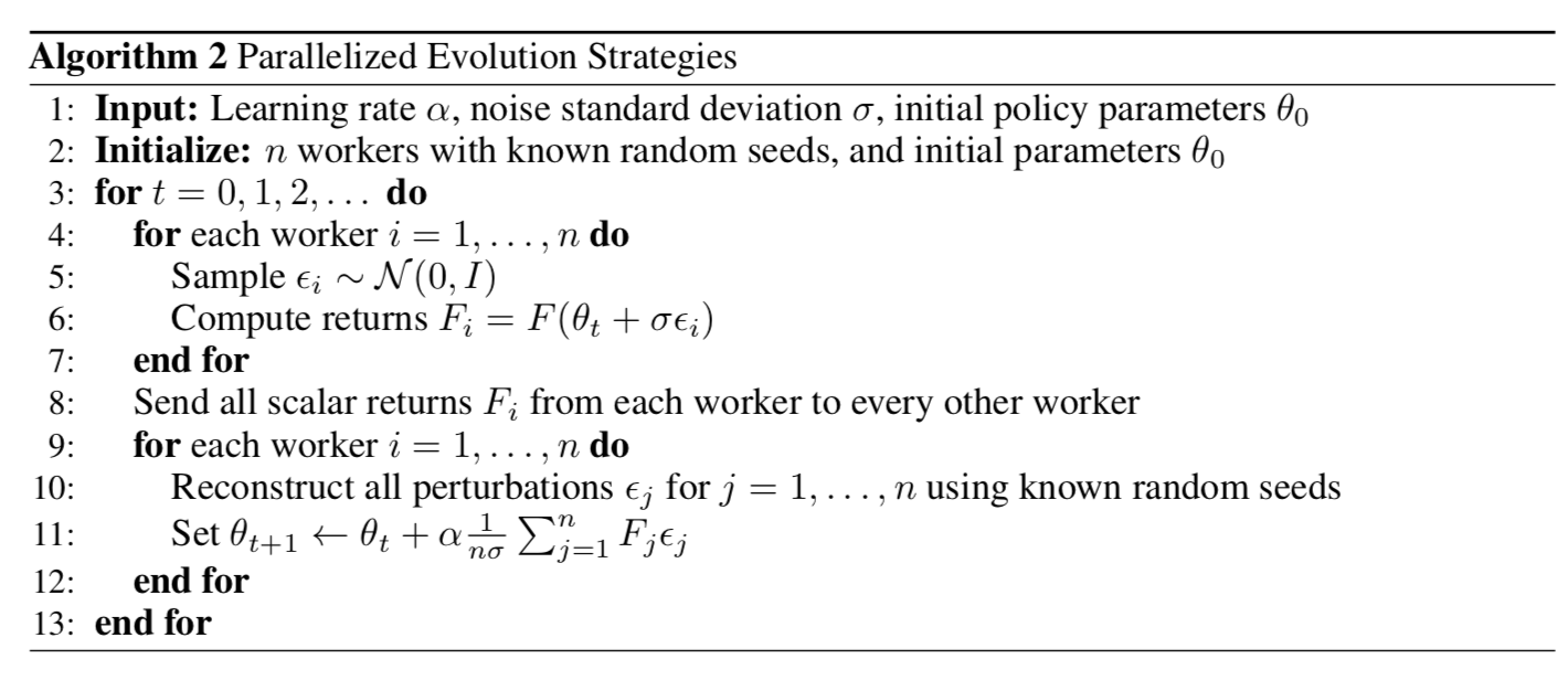
To improve robustness, OpenAI ES uses virtual batch normalization (BN with the mini-batch used for computing statistics held fixed), mirror sampling (evaluating a pair of $(-\epsilon, \epsilon)$), and fitness shaping.
Exploration with ES
Exploration (vs exploitation) is a central issue in RL. In the ES algorithm above, the optimization direction is inferred solely from the cumulative return $F(\theta)$. Without explicit exploration, an agent may become stuck in a local optimum.
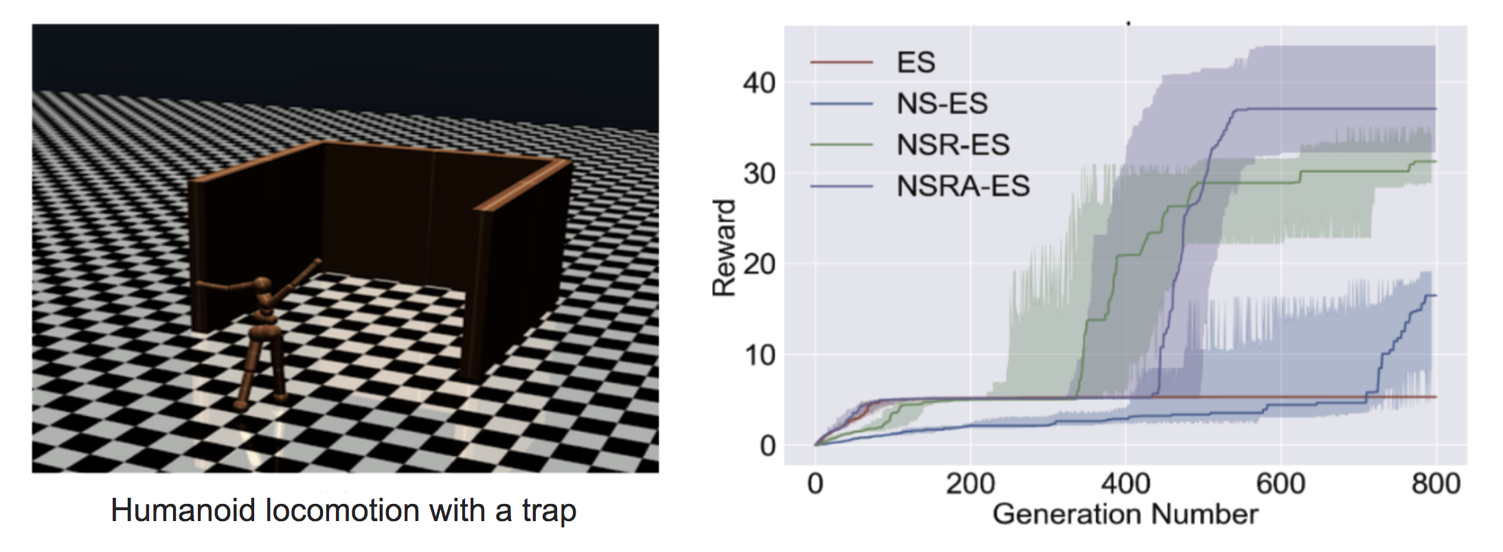
Novelty-Search ES (NS-ES; Conti et al, 2018) promotes exploration by updating parameters in the direction that maximizes a novelty score. This novelty score depends on a domain-specific behavior characterization function $b(\pi_\theta)$. The selection of $b(\pi_\theta)$ is task-dependent and can appear somewhat arbitrary; for example, in the paper’s Humanoid locomotion task, $b(\pi_\theta)$ is the final $(x,y)$ location of the agent.
- Each policy’s $b(\pi_\theta)$ is added to an archive set $\mathcal{A}$.
- The novelty of a policy $\pi_\theta$ is computed as the k-nearest-neighbor score between $b(\pi_\theta)$ and all other entries in $\mathcal{A}$. (The archive set use case is quite similar to episodic memory.)
The ES optimization step uses novelty rather than fitness:
NS-ES maintains a set of $M$ independently trained agents (a “meta-population”), $\mathcal{M} = \{\theta_1, \dots, \theta_M \}$, and advances one agent in proportion to its novelty score. Ultimately, the best policy is selected. This procedure is equivalent to ensembling; see the related idea in SVPG.
where $N$ is the number of Gaussian perturbation noise vectors and $\alpha$ is the learning rate.
NS-ES discards the reward function entirely and optimizes only novelty to avoid deceptive local optima. To reintroduce fitness into the formulation, two additional variants are proposed.
NSR-ES:
NSRAdapt-ES (NSRA-ES): the adaptive weighting parameter $w = 1.0$ initially. We begin decreasing $w$ if performance remains flat for a number of generations. When performance starts to improve, we stop decreasing $w$ and instead increase it. Under this schedule, fitness is emphasized when performance stagnates, while novelty is emphasized otherwise.
CEM-RL
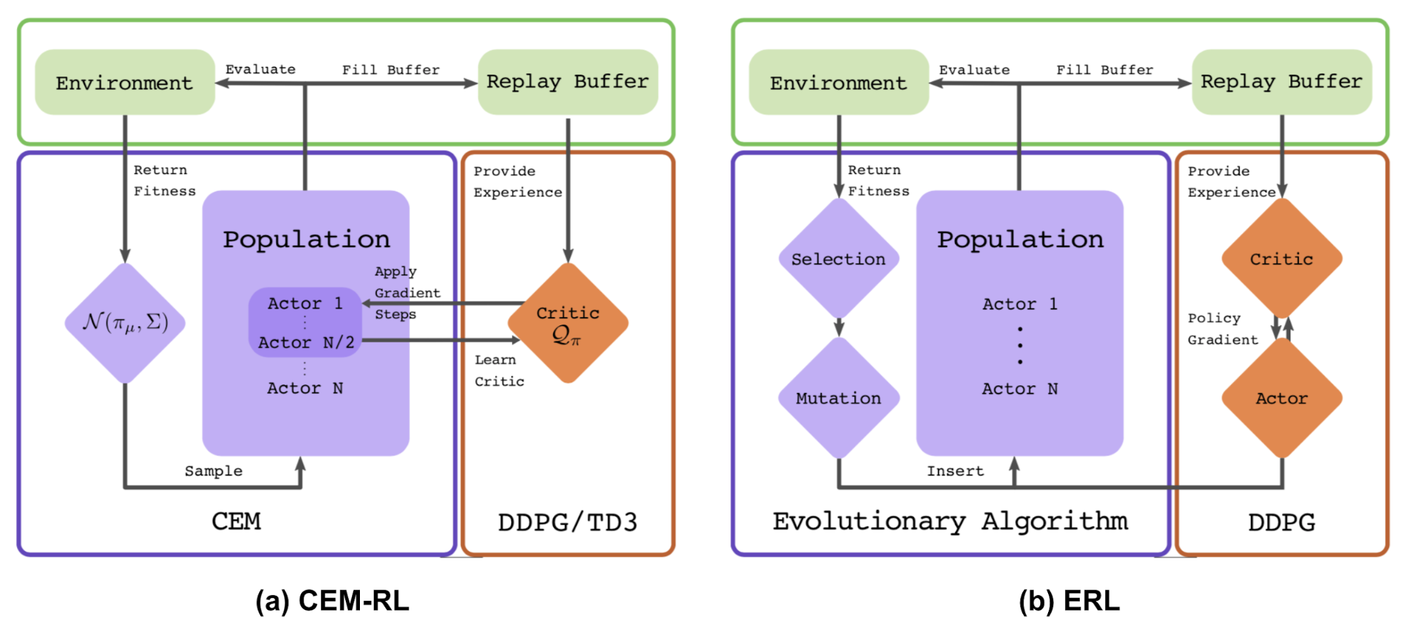
The CEM-RL method (Pourchot & Sigaud, 2019) combines the Cross Entropy Method (CEM) with either DDPG or TD3. Here, CEM behaves similarly to the simple Gaussian ES described above, and the same update can be replaced by CMA-ES. CEM-RL is built on the Evolutionary Reinforcement Learning (ERL; Khadka & Tumer, 2018) framework, in which a standard EA procedure selects and evolves a population of actors, and rollout experience produced during this process is added to the replay buffer for training both the RL-actor and RL-critic networks.
Workflow:
-
- The mean actor of the CEM population is $\pi_\mu$ is initialized with a random actor network.
-
- The critic network $Q$ is also initialized, and it will be updated by DDPG/TD3.
-
- Repeat until happy:
- a. Sample a population of actors $\sim \mathcal{N}(\pi_\mu, \Sigma)$.
- b. Evaluate half of the population. Their fitness scores are treated as the cumulative reward $R$ and added into the replay buffer.
- c. Update the other half jointly with the critic.
- d. Compute the new $\pi_mu$ and $\Sigma$ using the top-performing elite samples. CMA-ES can also be used for parameter updates.
Extension: EA in Deep Learning
(This section is not about evolution strategies, but it is still interesting and relevant.)
Evolutionary Algorithms have been applied to many deep learning problems. POET (Wang et al, 2019) is an EA-based framework that attempts to generate a range of different tasks while simultaneously solving the problems themselves. POET was discussed in my last post on meta-RL. Evolutionary Reinforcement Learning (ERL) is another example; see Fig. 7 (b).
Below, I introduce two applications in more detail: Population-Based Training (PBT) and Weight-Agnostic Neural Networks (WANN).
Hyperparameter Tuning: PBT
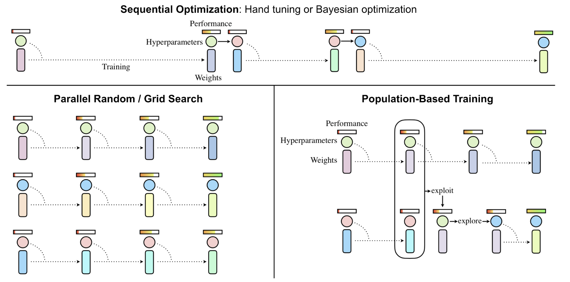
Population-Based Training (Jaderberg, et al, 2017), abbreviated PBT, applies EA to the problem of hyperparameter tuning. It jointly trains a population of models and their associated hyperparameters to achieve optimal performance.
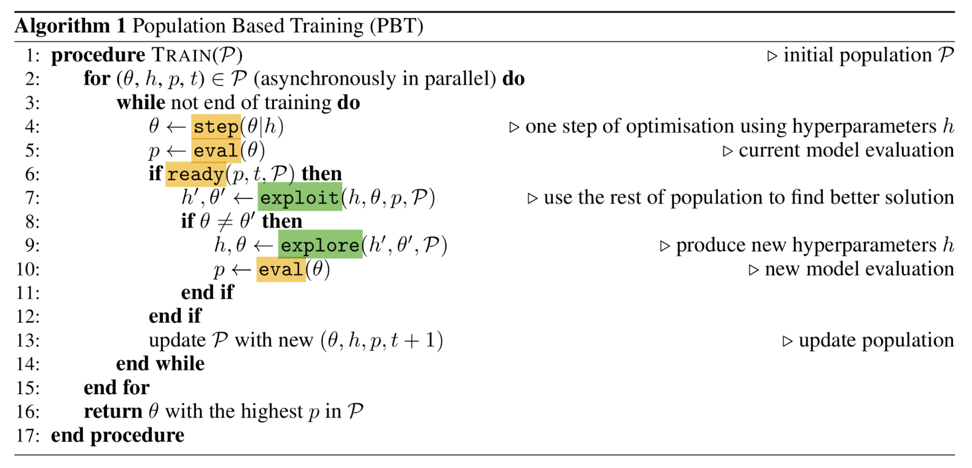
PBT begins with a set of random candidates, each consisting of an initialization of model weights paired with hyperparameters, $\{(\theta_i, h_i)\mid i=1, \dots, N\}$. Each sample is trained in parallel and asynchronously evaluates its performance at regular intervals. Whenever a member considers itself ready (for example, after taking enough gradient update steps, or once its performance is sufficiently good), it may be updated by comparing itself with the full population:
exploit(): If the model is underperforming, its weights may be replaced by those of a better-performing model.explore(): If the model weights are overwritten, theexplorestep perturbs the hyperparameters by adding random noise.
Through this process, only promising model and hyperparameter pairs survive and continue evolving, leading to more effective use of computational resources.
Network Topology Optimization: WANN
Weight Agnostic Neural Networks (abbreviated WANN; Gaier & Ha 2019) investigates how to search for the smallest network topologies that achieve optimal performance without training network weights. By disregarding the best configuration of network weights, WANN places substantially more emphasis on architecture itself, in contrast to NAS. WANN is strongly inspired by a classic genetic algorithm for evolving network topologies, NEAT (“Neuroevolution of Augmenting Topologies”; Stanley & Miikkulainen 2002).
The WANN workflow closely follows a standard GA:
- Initialize: Create a population of minimal networks.
- Evaluation: Test using a range of shared weight values.
- Rank and Selection: Rank by performance and complexity.
- Mutation: Generate a new population by perturbing the best networks.
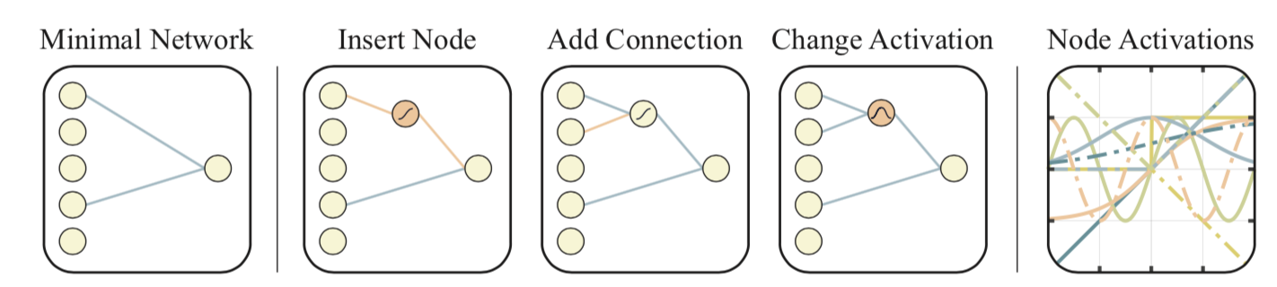
During the “evaluation” stage, all network weights are assigned the same value. In this way, WANN effectively searches for networks that can be described with minimal description length. During “selection,” both network connectivity and model performance are taken into account.
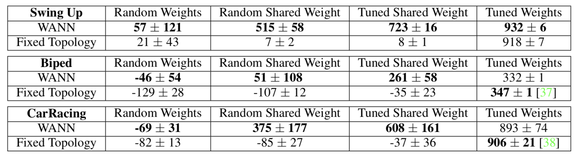
As shown in Fig. 11, WANN results are evaluated using both random weights and shared weights (a single shared weight). Notably, even under full weight-sharing and with only this single parameter tuned, WANN can identify topologies that achieve non-trivially strong performance.
Cited as:
@article{weng2019ES,
  title   = "Evolution Strategies",
  author  = "Weng, Lilian",
  journal = "lilianweng.github.io",
  year    = "2019",
  url     = "https://lilianweng.github.io/posts/2019-09-05-evolution-strategies/"
}
References
[1] Nikolaus Hansen. “The CMA Evolution Strategy: A Tutorial” arXiv preprint arXiv:1604.00772 (2016).
[2] Marc Toussaint. Slides: “Introduction to Optimization”
[3] David Ha. “A Visual Guide to Evolution Strategies” blog.otoro.net. Oct 2017.
[4] Daan Wierstra, et al. “Natural evolution strategies.” IEEE World Congress on Computational Intelligence, 2008.
[5] Agustinus Kristiadi. “Natural Gradient Descent” Mar 2018.
[6] Razvan Pascanu & Yoshua Bengio. “Revisiting Natural Gradient for Deep Networks.” arXiv preprint arXiv:1301.3584 (2013).
[7] Tim Salimans, et al. “Evolution strategies as a scalable alternative to reinforcement learning.” arXiv preprint arXiv:1703.03864 (2017).
[8] Edoardo Conti, et al. “Improving exploration in evolution strategies for deep reinforcement learning via a population of novelty-seeking agents.” NIPS. 2018.
[9] Aloïs Pourchot & Olivier Sigaud. “CEM-RL: Combining evolutionary and gradient-based methods for policy search.” ICLR 2019.
[10] Shauharda Khadka & Kagan Tumer. “Evolution-guided policy gradient in reinforcement learning.” NIPS 2018.
[11] Max Jaderberg, et al. “Population based training of neural networks.” arXiv preprint arXiv:1711.09846 (2017).
[12] Adam Gaier & David Ha. “Weight Agnostic Neural Networks.” arXiv preprint arXiv:1906.04358 (2019).