[Updated on 2020-02-03: mentioning PCG in the “Task-Specific Curriculum” section.
[Updated on 2020-02-04: Add a new “curriculum through distillation” section.

Trying to teach integration or differentiation to a 3-year-old who does not yet know basic arithmetic would feel impossible. This is precisely why education matters, it provides a structured way to break down sophisticated ideas and a well-designed curriculum that introduces concepts from easy to difficult. Curricula make hard things more approachable for humans. The parallel questions for machine learning are straightforward: can curricula train models more efficiently, and can we design curricula that accelerate learning?

In 1993, Jeffrey Elman proposed training neural networks using a curriculum. In early experiments on learning simple language grammar, he showed why this strategy matters: begin with a limited set of simple data and then gradually increase training-sample complexity; otherwise, the model may fail to learn entirely.

Relative to training without a curriculum, we would expect a curriculum to speed up convergence and to possibly, but not necessarily, improve final performance. Designing a curriculum that is both efficient and effective is difficult, and a poorly designed curriculum can even impede learning.

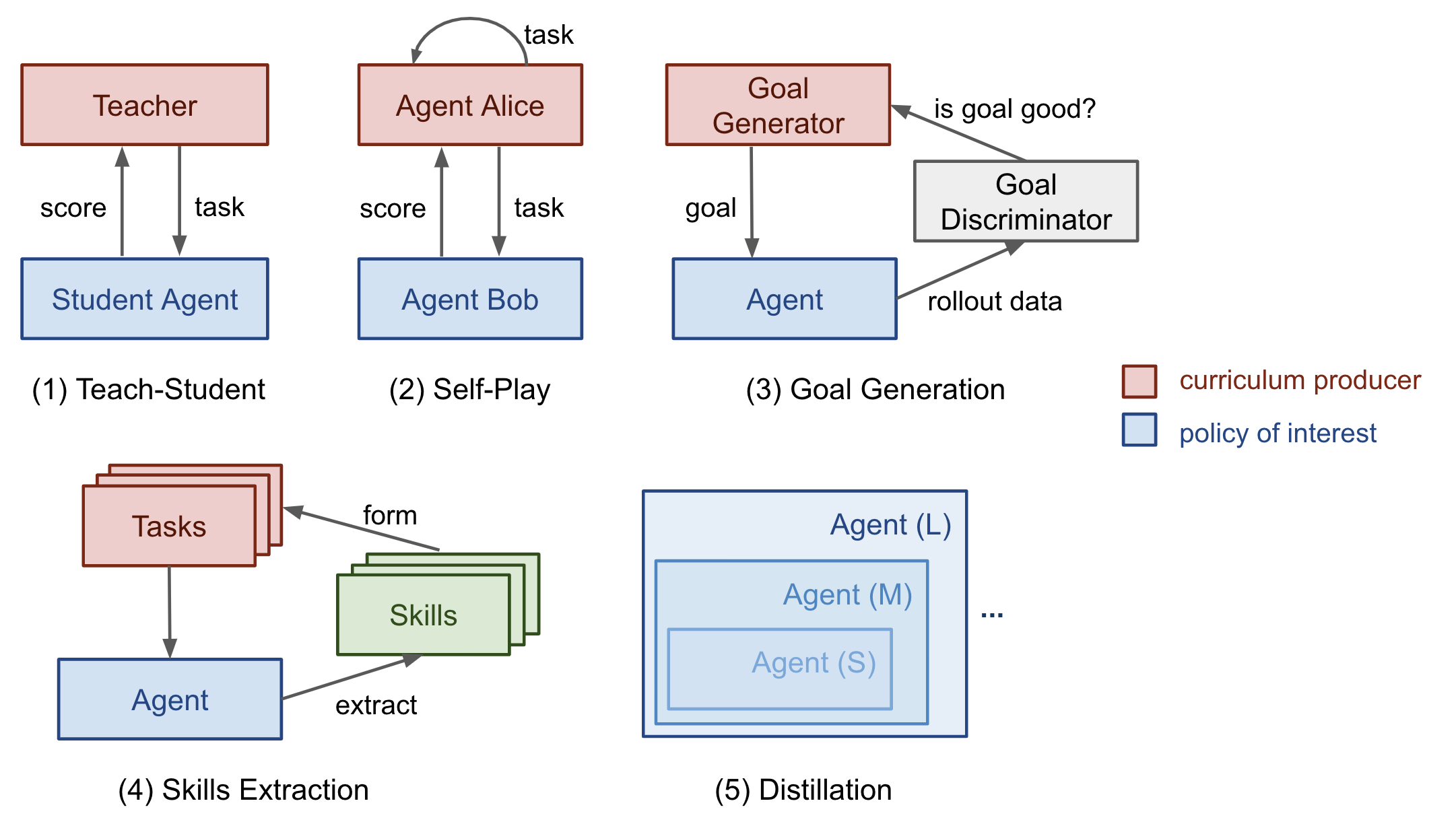
Next, we will examine several categories of curriculum learning. In most cases, these approaches are applied to Reinforcement Learning, with a few exceptions in Supervised Learning.

In “The importance of starting small” (Elman 1993), the opening lines are particularly memorable and, to me, both inspiring and moving:

“Humans differ from other species along many dimensions, but two are particularly noteworthy. Humans display an exceptional capacity to learn; and humans are remarkable for the unusually long time it takes to reach maturity. The adaptive advantage of learning is clear, and it may be argued that, through culture, learning has created the basis for a non-genetically based transmission of behaviors which may accelerate the evolution of our species.”

Indeed, learning may be the most powerful capability we have.

Task-Specific Curriculum

Bengio, et al. (2009) provides a solid overview of early curriculum learning work. The paper presented two ideas, supported by toy experiments using a manually designed, task-specific curriculum:

1. Cleaner Examples may yield better generalization faster.
2. Introducing gradually more difficult examples speeds up online training.

It is entirely plausible that some curriculum strategies are ineffective or even harmful. A central question for the field is: What general principles determine why some curriculum strategies work better than others? Bengio et al. (2009) hypothesized that learning benefits from emphasizing “interesting” examples, meaning those that are neither too difficult nor too trivial.

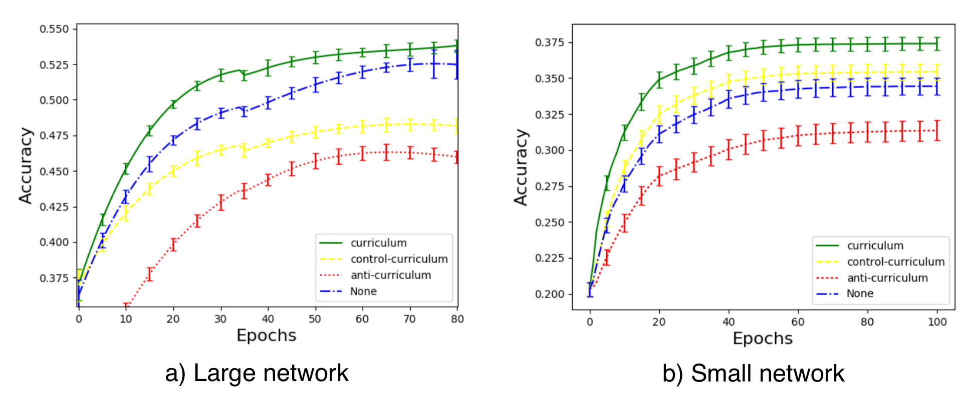
If a straightforward curriculum trains the model on samples with gradually increasing complexity, then we first need a way to quantify task difficulty. One approach is to measure difficulty via a sample’s minimal loss relative to another model, where that reference model has been pretrained on other tasks (Weinshall, et al. 2018). In this setup, the pretrained model’s knowledge can be transferred to the new model by using it to rank training samples. Fig. 2 illustrates the effectiveness of the curriculum group (green) compared with the control group (random order; yellow) and the anti group (reverse order; red).

Zaremba & Sutskever (2014) ran an interesting experiment: training an LSTM to predict the output of a short Python program for mathematical operations without executing the code. They found that a curriculum is necessary for learning. Program complexity is controlled by two parameters, length ∈ [1, a] and nesting∈ [1, b]. They evaluated three strategies:

1. Naive curriculum: increase length first until reaching a; then increase nesting and reset length to 1; repeat until both reach their maxima.
2. Mix curriculum: sample length ~ [1, a] and nesting ~ [1, b]
3. Combined: naive + mix.

They observed that the combined strategy always outperformed the naive curriculum, and it generally (though not always) outperformed the mix strategy. This suggests that mixing easy tasks into training is important to avoid forgetting.

Procedural content generation (PCG) is a widely used approach for producing video game content across a range of difficulty levels. PCG combines algorithmic randomness with substantial human expertise to design game elements and the dependencies between them. Procedurally generated levels have been incorporated into multiple benchmark environments to evaluate whether an RL agent can generalize to new levels it has not been trained on (meta-RL!), including GVGAI, OpenAI CoinRun, and the Procgen benchmark. Using GVGAI, Justesen, et al. (2018) showed that an RL policy can readily overfit to a specific game, while training with a simple curriculum that increases task difficulty as the model improves can enhance generalization to new human-designed levels. Similar findings appear in CoinRun (Cobbe, et al. 2018). POET (Wang et al, 2019) is another example that uses an evolutionary algorithm together with procedurally generated game levels to improve RL generalization; I described it in more detail in my meta-RL post.

To apply the curriculum learning approaches above, we typically must resolve two practical issues during training:

1. Define a metric that quantifies task difficulty, enabling tasks to be ordered accordingly.
2. Provide the model with a sequence of tasks whose difficulty increases over training.

However, task order does not need to be strictly sequential. In our Rubik’s cube paper (OpenAI et al, 2019), we relied on Automatic domain randomization (ADR) to construct a curriculum by expanding a distribution over environments with increasing complexity. Each task’s difficulty (solving a Rubik’s cube across a set of environments) is determined by the randomization ranges of multiple environmental parameters. Even under the simplified assumption that all environmental parameters are uncorrelated, we were able to build a useful curriculum that enabled our robot hand to learn the task.

Teacher-Guided Curriculum

The idea of Automatic Curriculum Learning was introduced slightly earlier by Graves, et al. 2017. It treats a $N$-task curriculum as an $N$-armed bandit problem and learns an adaptive policy that optimizes returns from this bandit.

The paper considers two categories of learning signals:

1. Loss-driven progress: the change in the loss function before versus after a single gradient update. This reward signal tracks learning speed, since the largest loss reduction corresponds to the fastest learning.
2. Complex-driven progress: the KL divergence between the posterior and prior distributions over network weights. This signal is inspired by the MDL principle: “increasing the model complexity by a certain amount is only worthwhile if it compresses the data by a greater amount”. Under this view, model complexity should increase most when the model generalizes well to training examples.

This approach, automatically proposing curricula via an additional RL agent, was formalized as Teacher-Student Curriculum Learning (TSCL; Matiisen, et al. 2017). In TSCL, the student is the RL agent learning the actual tasks, while the teacher is a task-selection policy. The student seeks to master a complex task that may be difficult to learn directly; to make learning easier, the teacher guides training by selecting appropriate subtasks.

During training, the student should focus on tasks that:

1. enable the fastest learning progress; or
2. are in danger of being forgotten.

Note: Framing the teacher model as an RL problem feels quite similar to Neural Architecture Search (NAS). However, in TSCL the RL model operates over the task space, whereas NAS operates over the architecture space of the primary model.

Training the teacher is formulated as a POMDP:

• The unobserved $s_t$ is the full state of the student model.
• The observed $o = (x_t^{(1)}, \dots, x_t^{(N)})$ are a list of scores for $N$ tasks.
• The action $a$ is to pick on subtask.
• The reward per step is the score delta.$r_t = \sum_{i=1}^N x_t^{(i)} - x_{t-1}^{(i)}$ (i.e., equivalent to maximizing the score of all tasks at the end of the episode).

Estimating learning progress from noisy task scores, while balancing exploration and exploitation, can borrow methods from non-stationary multi-armed bandits, such as ε-greedy or Thompson sampling.

The core idea can be summarized as using one policy to propose tasks so that another policy can learn more effectively. Interestingly, both of the works above (in discrete task spaces) found that uniformly sampling tasks is a surprisingly strong baseline.

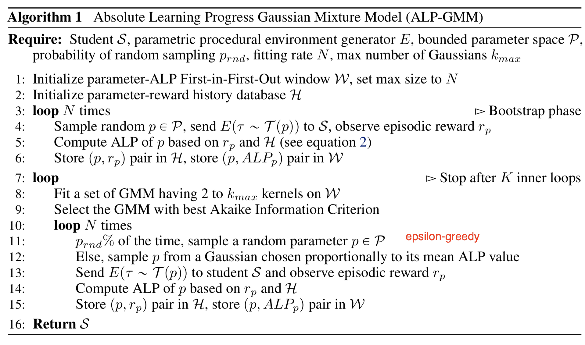
What if the task space is continuous? Portelas, et al. (2019) studied a continuous teacher-student framework in which the teacher samples parameters from a continuous task space to build a curriculum. For a newly sampled parameter $p$, the absolute learning progress (ALP) is measured as $\text{ALP}_p = \vert r - r_\text{old} \vert$, where $r$ is the episodic reward associated with $p$ and $r_\text{old}$ is the reward associated with $p_\text{old}$. Here, $p_\text{old}$ is the previously sampled parameter closest to $p$ in task space, retrieved via nearest neighbor. Note how ALP differs from the learning signals in TSCL or Grave, et al. 2017 above: ALP measures the reward difference between two tasks, rather than the performance difference across two time steps on the same task.

On top of the task-parameter space, a Gaussian mixture model (GMM) is trained to fit the distribution of $\text{ALP}_p$ over $p$. Task sampling uses ε-greedy: with some probability it samples a random task, otherwise it samples from the GMM proportionally to ALP.

Curriculum through Self-Play

Unlike the teacher-student setup, where the teacher selects tasks for the student without knowledge of task content, we can instead ask: what if both agents train directly on the main task? Further, what if they compete?

Sukhbaatar, et al. (2017) proposed an automatic curriculum framework based on asymmetric self-play. Two agents, Alice and Bob, operate in the same task but with different objectives: Alice sets challenges by reaching a state, and Bob attempts to reach that same state as quickly as possible.

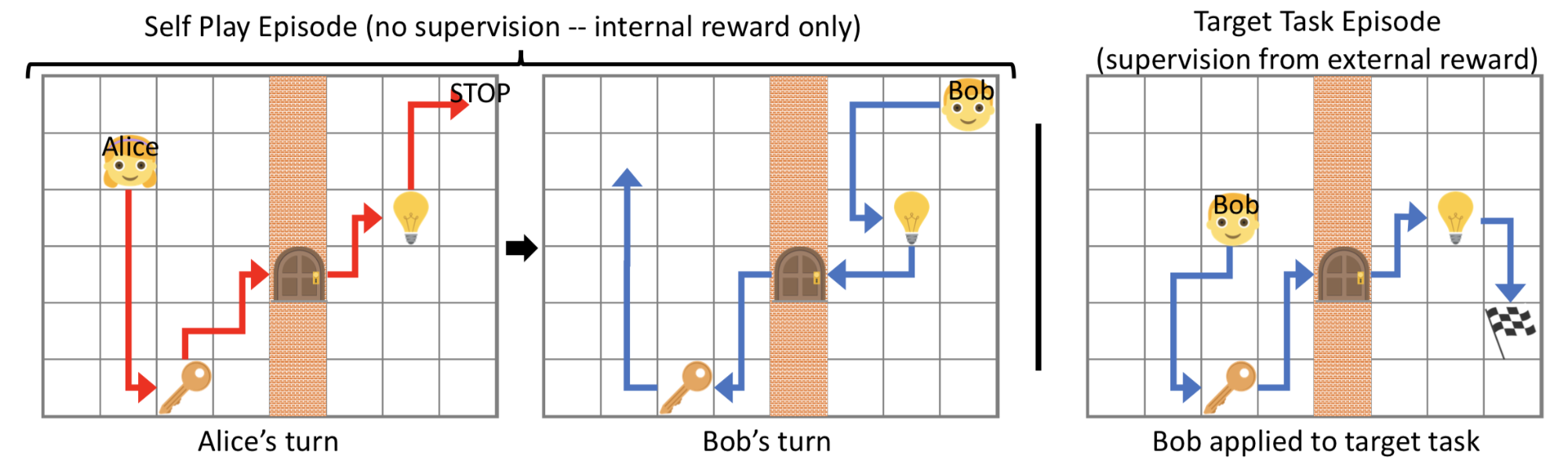
Consider Alice and Bob as two distinct instances of an RL agent interacting with the same environment, but with different parameters and different loss objectives. Training via self-play uses two episode types:

• In a self-play episode, Alice changes the environment state from $s_0$ to $s_t$, and Bob is then asked to return the environment to its original state $s_0$ to receive an internal reward.
• In a target task episode, Bob receives an external reward if he reaches the target flag.

Because B must repeat actions between the same pair of $(s_0, s_t)$ of A, this approach applies only to reversible or resettable environments.

Alice should learn to push Bob beyond his comfort zone without proposing impossible challenges. Bob’s reward is defined as $R_B = -\gamma t_B$ and Alice’s reward as $R_A = \gamma \max(0, t_B - t_A)$, where $t_B$ is the total time for B to complete the task, $t_A$ is the time until Alice takes the STOP action, and $\gamma$ is a scalar constant that rescales the reward to be comparable to the external task reward. If B fails a task, $t_B = t_\max - t_A$. Both policies are goal-conditioned. The resulting losses imply:

1. B wants to finish a task asap.
2. A prefers tasks that take more time of B.
3. A does not want to take too many steps when B is failing.

Through this interaction, Alice and Bob automatically construct a curriculum of progressively more challenging tasks. At the same time, because Alice completes the task before assigning it to Bob, solvability is ensured.

The pattern of A proposing tasks and B solving them resembles the Teacher-Student framework. However, in asymmetric self-play, Alice (acting as a teacher) also performs the same task to identify challenging cases for Bob, rather than explicitly optimizing Bob’s learning process.

Automatic Goal Generation

RL policies often need to perform well across a set of tasks. Goals should be selected so that, at each stage of training, they are neither too difficult nor too easy for the current policy. A goal $g \in \mathcal{G}$ can be defined as a set of states $S^g$, and the goal is achieved whenever the agent reaches any of those states.

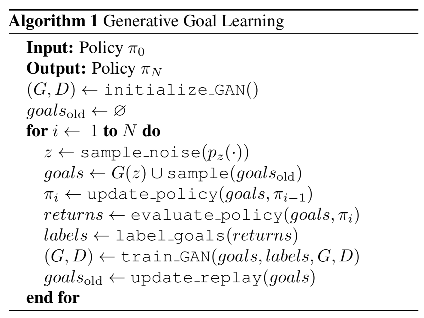
Generative Goal Learning (Florensa, et al. 2018) uses a Goal GAN to automatically generate goals. In their experiments, rewards are very sparse: a single binary indicator of whether a goal is achieved. The policy is goal-conditioned:

Here $R^g(\pi)$ is the expected return, which is also the success probability. Given trajectories sampled from the current policy, the return is positive as long as any visited state belongs to the goal set.

The method iterates the following three steps until the policy converges:

1. Label a set of goals based on whether they match the current policy’s appropriate difficulty range.

• Goals at an appropriate difficulty level are called GOID (short for “Goals of Intermediate Difficulty”).
  $\text{GOID}_i := \{g : R_\text{min} \leq R^g(\pi_i) \leq R_\text{max} \} \subseteq G$
• Here $R_\text{min}$ and $R_\text{max}$ can be interpreted as minimum and maximum probabilities of reaching a goal over T time-steps.

2. Train a Goal GAN model on the labeled goals from step 1 to generate new goals
3. Train the policy on these generated goals, improving its coverage objective.

The Goal GAN produces an automatic curriculum:

• Generator $G(z)$: proposes a new goal. => expected to be uniformly sampled from the $GOID$ set.
• Discriminator $D(g)$: evaluates whether a goal is achievable. => expected to determine whether a goal belongs to the $GOID$ set.

The Goal GAN follows the LSGAN (Least-Squared GAN; Mao et al., (2017)) design, which is more stable than the vanilla GAN. Under LSGAN, we minimize the following losses for $D$ and $G$, respectively:

where $a$ is the label for fake data, $b$ for real data, and $c$ is the value that $G$ wants $D$ to believe for fake data. In the LSGAN experiments, they used $a=-1, b=1, c=0$.

The Goal GAN adds an additional binary flag $y_b$ indicating whether a goal $g$ is real ($y_g = 1$) or fake ($y_g = 0$), enabling training with negative samples:

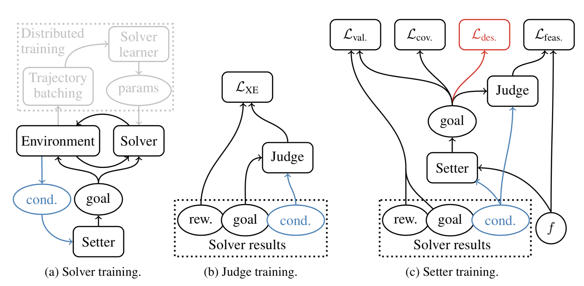
Building on this idea, Racaniere & Lampinen, et al. (2019) proposed a method that makes the goal generator’s objective more sophisticated. As in generative goal learning, their method uses three components:

• Solver/Policy $\pi$: At the start of each episode, the solver receives a goal $g$ and receives a single binary reward $R^g$ at the end.
• Judge/Discriminator $D(.)$: A classifier that predicts the binary reward (whether the goal is achievable). More precisely, it outputs the logit of the probability of achieving the given goal, $\sigma(D(g)) = p(R^g=1\vert g)$, where $\sigma$ is the sigmoid function.
• Setter/Generator $G(.)$: The setter takes a desired feasibility score $f \in \text{Unif}(0, 1)$ as input and generates $g = G(z, f)$, where the latent variable $z$ is sampled by $z \sim \mathcal{N}(0, I)$. The goal generator is designed to reversible, so $G^{-1}$ can map backwards from a goal $g$ to a latent $z = G^{-1}(g, f)$

The generator is trained with three objectives:

1. Goal validity: The generated goal should be achievable by an expert policy. The corresponding generative loss increases the likelihood of producing goals that the solver has achieved previously (as in HER).
   • $\mathcal{L}_\text{val}$ is the negative log-likelihood of generated goals that have been solved by the solver in the past.

2. Goal feasibility: The generated goal should be achievable by the current policy, meaning its difficulty should be appropriate.
   • $\mathcal{L}_\text{feas}$ is the probability output of the judge model $D$ for the generated goal $G(z, f)$, and it should match the desired $f$.

3. Goal coverage: Maximize the entropy of generated goals to promote diversity and improve coverage of the goal space.

Their experiments indicated that complex environments require all three losses above. When the environment changes between episodes, both the goal generator and the discriminator must be conditioned on environmental observation to achieve better results. If a desired goal distribution is available, an additional loss can be introduced to match that distribution via Wasserstein distance. With this loss, the generator can guide the solver toward mastering the intended tasks more efficiently.

Skill-Based Curriculum

Another perspective is to decompose what an agent can accomplish into a set of skills, where each skill set can be mapped to a task. Suppose an agent interacts with an environment in an unsupervised way. Can we discover useful skills from that interaction and then assemble them, through a curriculum, into solutions for more complex tasks?

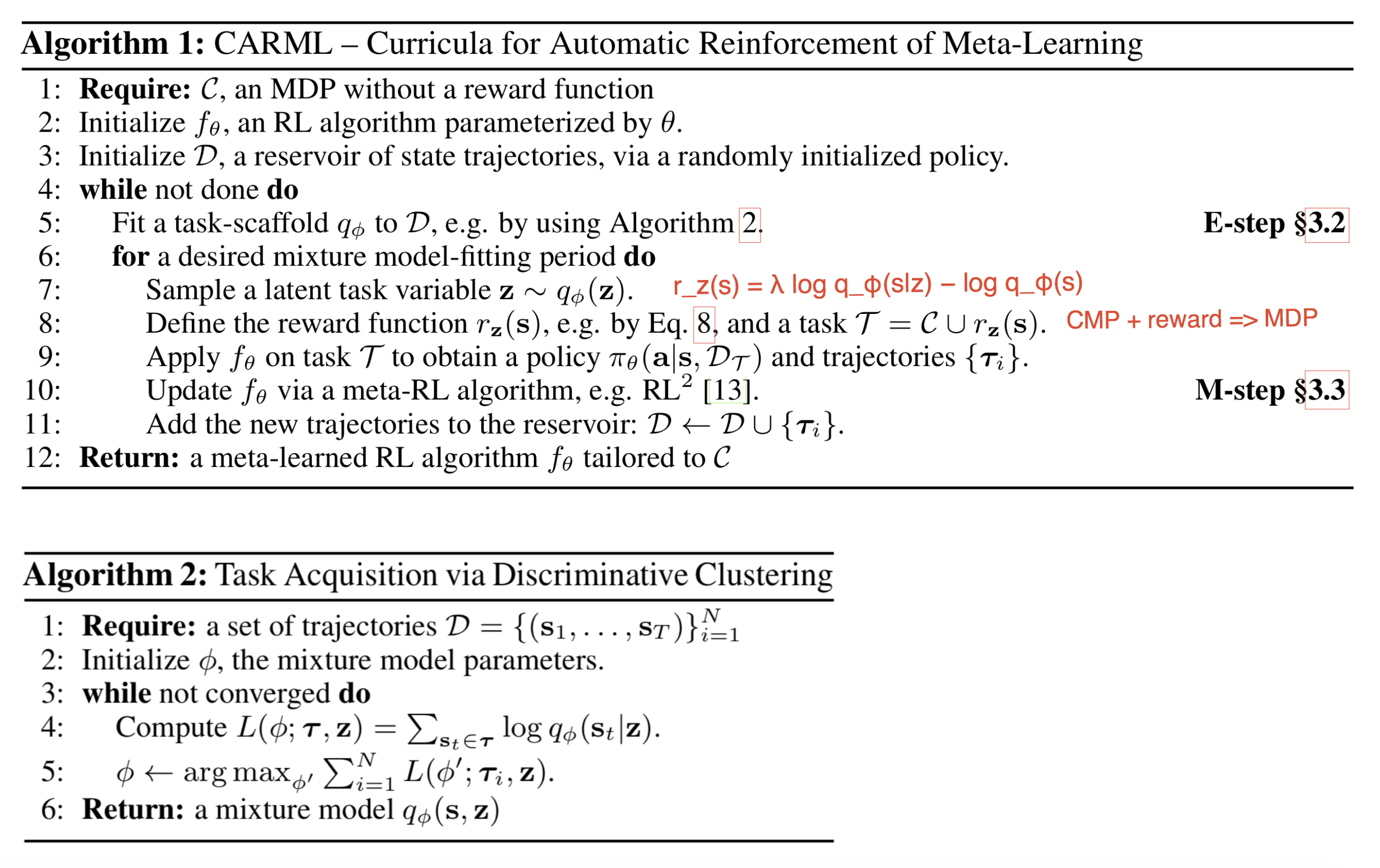
Jabri, et al. (2019) proposed an automatic curriculum called CARML (short for “Curricula for Unsupervised Meta-Reinforcement Learning”). CARML models unsupervised trajectories in a latent skill space, with the goal of training meta-RL policies (that is, policies that can transfer to unseen tasks). CARML’s training-environment setup resembles DIAYN. However, CARML is trained from pixel-level observations, whereas DIAYN operates on the true state space. An RL algorithm $\pi_\theta$, parameterized by $\theta$, is trained through unsupervised interaction framed as a CMP, combined with a learned reward function $r$. This configuration naturally supports meta-learning, since a customized reward function can be supplied only at test time.

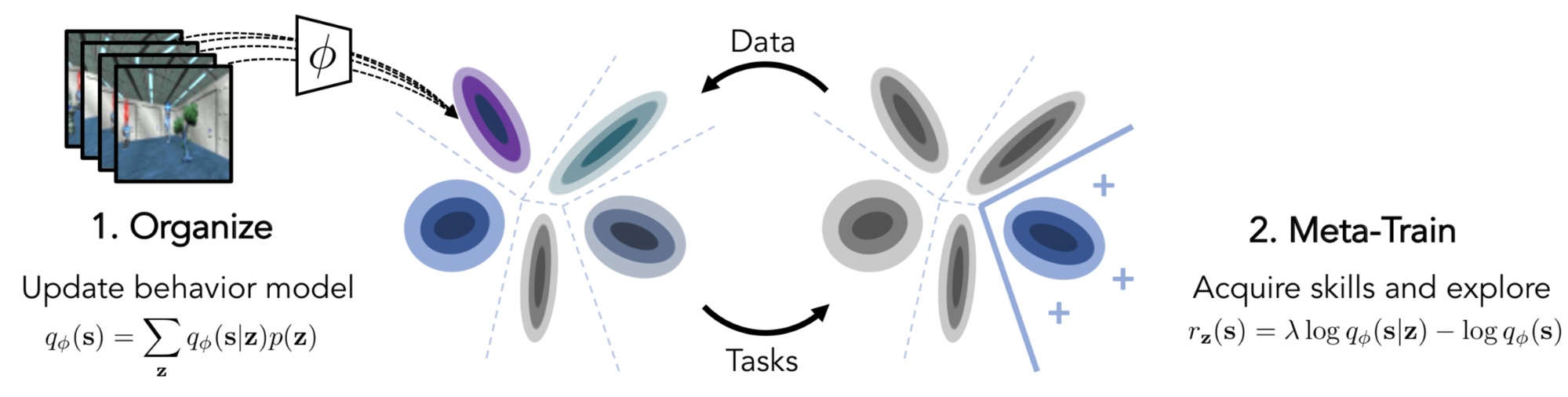
CARML is formulated as a variational Expectation-Maximization (EM) procedure.

(1) E-Step: This phase organizes experiential data. Collected trajectories are modeled as a mixture of latent components that form the basis of skills.

Let $z$ denote a latent task variable, and let $q_\phi$ denote a variational distribution over $z$. This distribution may be implemented as a mixture model with discrete $z$ or as a VAE with continuous $z$. The variational posterior $q_\phi(z \vert s)$ effectively behaves like a classifier that predicts a skill from a state. Our objective is to maximize $q_\phi(z \vert s)$ so that it distinguishes, as strongly as possible, between data generated by different skills. During the E-step, $q_\phi$ is fit using a set of trajectories produced by $\pi_\theta$.

More precisely, given a trajectory $\tau = (s_1,\dots,s_T)$, we seek $\phi$ such that:

A simplifying assumption is applied here: the ordering of states within a trajectory is ignored.

(2) M-Step: This phase performs meta-RL training with $\pi_\theta$. The learned skill space is treated as the training task distribution. CARML is agnostic to which meta-RL algorithm is used to update policy parameters.

Given a trajectory $\tau$, it is natural for the policy to maximize the mutual information between $\tau$ and $z$, $I(\tau;z) = H(\tau) - H(\tau \vert z)$, because:

• maximizing $H(\tau)$ => promotes diversity in the policy data space; this quantity is expected to be large.
• minimizing $H(\tau \vert z)$ => constrains behavior when conditioned on a particular skill; this quantity is expected to be small.

This yields:

Accordingly, we can choose the reward to be $\log q_\phi(s \vert z) - \log q_\phi(s)$, as indicated by the red portion of the equation above. To trade off task-specific exploration (as shown in red below) against latent skill matching (as shown in blue below), we introduce a parameter $\lambda \in [0, 1]$. Each realization of $z \sim q_\phi(z)$ induces a reward function $r_z(s)$ (recall: reward + CMP => MDP) as follows:

A latent skill space can be learned in multiple ways, for example as in Hausman, et al. 2018. Their method aims to learn a task-conditioned policy, $\pi(a \vert s, t^{(i)})$, where $t^{(i)}$ is drawn from a discrete list of $N$ tasks, $\mathcal{T} = [t^{(1)}, \dots, t^{(N)}]$. However, instead of learning $N$ separate solutions (one per task), it is preferable to learn a latent skill space in which each task is represented as a distribution over skills, enabling skills to be reused between tasks. The policy is defined as $\pi_\theta(a \vert s,t) = \int \pi_\theta(a \vert z,s,t) p_\phi(z \vert t)\mathrm{d}z$, where $\pi_\theta$ and $p_\phi$ are the policy and embedding networks to be learned, respectively. If $z$ is discrete (that is, sampled from a set of $K$ skills), then the policy becomes a mixture of $K$ sub-policies. Policy training uses SAC, and the dependence on $z$ is incorporated into the entropy term.

Curriculum through Distillation

[I debated the name of this section for a while, considering cloning, inheritance, and distillation. In the end, I chose distillation because it sounds the coolest B-)]

The progressive neural network architecture (Rusu et al. 2016) is motivated by the need to transfer learned skills efficiently across tasks while avoiding catastrophic forgetting. The curriculum is implemented via a set of neural network towers that are stacked progressively (referred to as “columns” in the paper).

A progressive network is organized as follows:

1. Training begins with a single column containing $L$ neuron layers, with corresponding activation layers labeled $h^{(1)}_i, i=1, \dots, L$. This single-column network is trained on one task until convergence, resulting in the parameter configuration $\theta^{(1)}$.

2. After switching to the next task, a new column is added to adapt to the new setting, while $\theta^{(1)}$ is frozen to preserve skills learned on the previous task. The new column has activation layers labeled $h^{(2)}_i, i=1, \dots, L$ and parameters $\theta^{(2)}$.

3. Step 2 is repeated for each additional task. The $i$-th layer activation in the $k$-th column depends on the preceding activation layers from all existing columns:

   $ h^{(k)}_i = f(W^{(k)}_i h^{(k)}_{i-1} + \sum_{j < k} U_i^{(k:j)} h^{(j)}_{i-1}) $

   where $W^{(k)}_i$ is the weight matrix for layer $i$ in column $k$; $U_i^{(k:j)}, j < k$ are the weight matrices that project layer $i-1$ of column $j$ into layer $i$ of column $k$ ($ j < k $). The weight matrices above are learned. $f(.)$ is a user-chosen non-linear activation function.

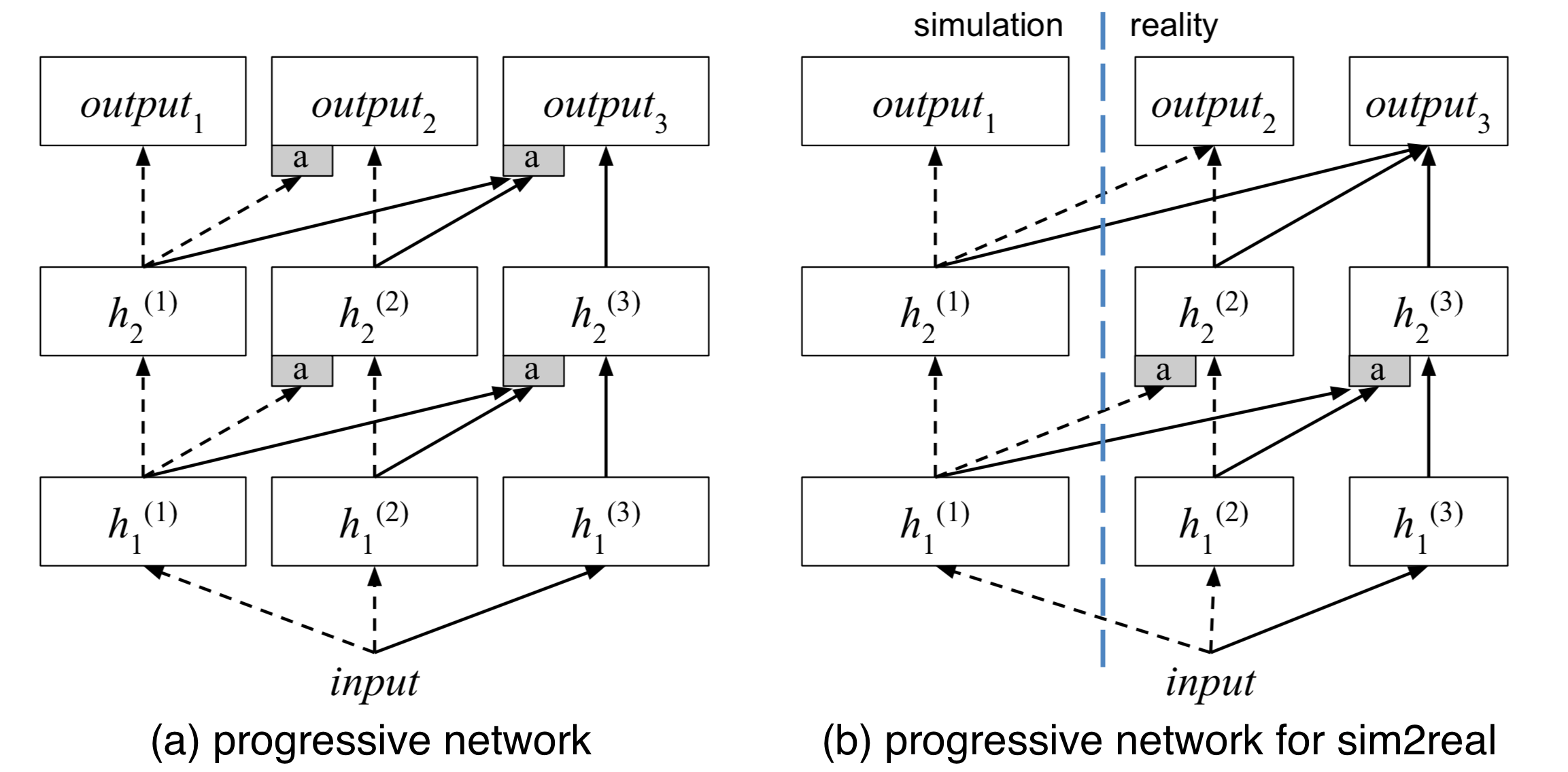
The paper evaluated Atari games by training a progressive network across multiple games to test whether features learned in one game transfer to another. They do. Notably, however, strong reliance on features from earlier columns does not always correlate with good transfer performance on the new task. One hypothesis is that features from the old task may bias learning on the new task, causing the policy to become stuck in a sub-optimal solution. Overall, the progressive network outperforms approaches that fine-tune only the top layer, and it can achieve transfer performance comparable to fine-tuning the full network.

One application of progressive networks is sim2real transfer (Rusu, et al. 2017): the first column is trained in simulation using many samples, and then additional columns (potentially corresponding to different real-world tasks) are appended and trained using only a small amount of real data.

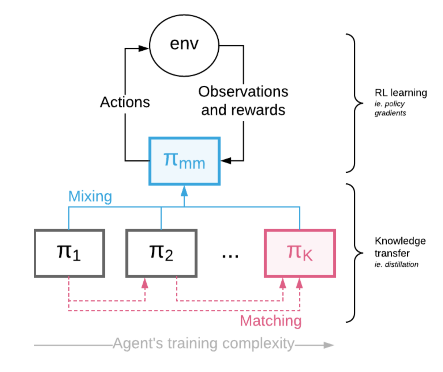
Czarnecki, et al. (2018) introduced another RL training framework, Mix & Match (abbreviated M&M), which provides a curriculum by copying knowledge between agents. Consider a sequence of agents from simple to complex, $\pi_1, \dots, \pi_K$, each parameterized with some shared weights (for example, by sharing lower layers). M&M trains a mixture of agents, although only the final performance of the most complex agent, $\pi_K$, is used for evaluation.

Concurrently, M&M learns a categorical distribution $c \sim \text{Categorical}(1, \dots, K \vert \alpha)$ with pmf $p(c=i) = \alpha_i$, representing the probability of selecting a given policy at a particular time. The mixed M&M policy is a straightforward weighted sum: $\pi_\text{mm}(a \vert s) = \sum_{i=1}^K \alpha_i \pi_i(a \vert s)$. Curriculum learning is achieved by dynamically adjusting $\alpha_i$ from $\alpha_K=0$ to $\alpha_K=1$. Tuning $\alpha$ may be done manually or via population-based training.

To promote cooperation rather than competition among policies, M&M adds an additional distillation-style loss $\mathcal{L}_\text{mm}(\theta)$ on top of the RL loss $\mathcal{L}_\text{RL}$. The knowledge transfer loss $\mathcal{L}_\text{mm}(\theta)$ computes the KL divergence between two policies, $\propto D_\text{KL}(\pi_{i}(. \vert s) | \pi_j(. \vert s))$ for $i < j$. This term encourages more complex agents to match simpler agents early in training. The resulting total loss is $\mathcal{L} = \mathcal{L}_\text{RL}(\theta \vert \pi_\text{mm}) + \lambda \mathcal{L}_\text{mm}(\theta)$.

Citation

Cited as:

Weng, Lilian. (Jan 2020). Curriculum for reinforcement learning. Lil’Log. https://lilianweng.github.io/posts/2020-01-29-curriculum-rl/.

Or

@article{weng2020curriculum,
  title   = "Curriculum for Reinforcement Learning",
  author  = "Weng, Lilian",
  journal = "lilianweng.github.io",
  year    = "2020",
  month   = "Jan",
  url     = "https://lilianweng.github.io/posts/2020-01-29-curriculum-rl/"
}

References

[1] Jeffrey L. Elman. “Learning and development in neural networks: The importance of starting small.” Cognition 48.1 (1993): 71-99.

[2] Yoshua Bengio, et al. “Curriculum learning.” ICML 2009.

[3] Daphna Weinshall, Gad Cohen, and Dan Amir. “Curriculum learning by transfer learning: Theory and experiments with deep networks.” ICML 2018.

[4] Wojciech Zaremba and Ilya Sutskever. “Learning to execute.” arXiv preprint arXiv:1410.4615 (2014).

[5] Tambet Matiisen, et al. “Teacher-student curriculum learning.” IEEE Trans. on neural networks and learning systems (2017).

[6] Alex Graves, et al. “Automated curriculum learning for neural networks.” ICML 2017.

[7] Remy Portelas, et al. Teacher algorithms for curriculum learning of Deep RL in continuously parameterized environments. CoRL 2019.

[8] Sainbayar Sukhbaatar, et al. “Intrinsic Motivation and Automatic Curricula via Asymmetric Self-Play.” ICLR 2018.

[9] Carlos Florensa, et al. “Automatic Goal Generation for Reinforcement Learning Agents” ICML 2019.

[10] Sebastien Racaniere & Andrew K. Lampinen, et al. “Automated Curriculum through Setter-Solver Interactions” ICLR 2020.

[11] Allan Jabri, et al. “Unsupervised Curricula for Visual Meta-Reinforcement Learning” NeuriPS 2019.

[12] Karol Hausman, et al. “Learning an Embedding Space for Transferable Robot Skills “ ICLR 2018.

[13] Josh Merel, et al. “Reusable neural skill embeddings for vision-guided whole body movement and object manipulation” arXv preprint arXiv:1911.06636 (2019).

[14] OpenAI, et al. “Solving Rubik’s Cube with a Robot Hand.” arXiv preprint arXiv:1910.07113 (2019).

[15] Niels Justesen, et al. “Illuminating Generalization in Deep Reinforcement Learning through Procedural Level Generation” NeurIPS 2018 Deep RL Workshop.

[16] Karl Cobbe, et al. “Quantifying Generalization in Reinforcement Learning” arXiv preprint arXiv:1812.02341 (2018).

[17] Andrei A. Rusu et al. “Progressive Neural Networks” arXiv preprint arXiv:1606.04671 (2016).

[18] Andrei A. Rusu et al. “Sim-to-Real Robot Learning from Pixels with Progressive Nets.” CoRL 2017.

[19] Wojciech Marian Czarnecki, et al. “Mix & Match – Agent Curricula for Reinforcement Learning.” ICML 2018.