The Transformer Family
[Updated on 2023-01-27: After nearly three years, I completed a major refactoring of this post to incorporate a number of new Transformer models released since 2020. The revised and expanded version of this post is available here: The Transformer Family Version 2.0. Please refer to that post for this topic.]
· 25 min read · Curated and presented by Arthur Sedek
[Updated on 2023-01-27: After almost three years, I did a big refactoring update of this post to incorporate a bunch of new Transformer models since 2020. The enhanced version of this post is here: The Transformer Family Version 2.0. Please refer to that post on this topic.]
It has been nearly two years since my previous post on attention. The rapid progress in new and improved Transformer variants has prompted me to write another focused article, centered on how the vanilla Transformer can be upgraded to provide a longer-term attention span, lower memory and compute costs, better RL task solving, and additional improvements.
Notations
| Symbol | Meaning |
|---|---|
| $d$ | The model size / hidden state dimension / positional encoding size. |
| $h$ | The number of heads in multi-head attention layer. |
| $L$ | The segment length of input sequence. |
| $\mathbf{X} \in \mathbb{R}^{L \times d}$ | The input sequence where each element has been mapped into an embedding vector of shape $d$, same as the model size. |
| $\mathbf{W}^k \in \mathbb{R}^{d \times d_k}$ | The key weight matrix. |
| $\mathbf{W}^q \in \mathbb{R}^{d \times d_k}$ | The query weight matrix. |
| $\mathbf{W}^v \in \mathbb{R}^{d \times d_v}$ | The value weight matrix. Often we have $d_k = d_v = d$. |
| $\mathbf{W}^k_i, \mathbf{W}^q_i \in \mathbb{R}^{d \times d_k/h}; \mathbf{W}^v_i \in \mathbb{R}^{d \times d_v/h}$ | The weight matrices per head. |
| $\mathbf{W}^o \in \mathbb{R}^{d_v \times d}$ | The output weight matrix. |
| $\mathbf{Q} = \mathbf{X}\mathbf{W}^q \in \mathbb{R}^{L \times d_k}$ | The query embedding inputs. |
| $\mathbf{K} = \mathbf{X}\mathbf{W}^k \in \mathbb{R}^{L \times d_k}$ | The key embedding inputs. |
| $\mathbf{V} = \mathbf{X}\mathbf{W}^v \in \mathbb{R}^{L \times d_v}$ | The value embedding inputs. |
| $S_i$ | A collection of key positions for the $i$-th query $\mathbf{q}_i$ to attend to. |
| $\mathbf{A} \in \mathbb{R}^{L \times L}$ | The self-attention matrix between a input sequence of length $L$ and itself. $\mathbf{A} = \text{softmax}(\mathbf{Q}\mathbf{K}^\top / \sqrt{d_k})$. |
| $a_{ij} \in \mathbf{A}$ | The scalar attention score between query $\mathbf{q}_i$ and key $\mathbf{k}_j$. |
| $\mathbf{P} \in \mathbb{R}^{L \times d}$ | position encoding matrix, where the $i$-th row $\mathbf{p}_i$ is the positional encoding for input $\mathbf{x}_i$. |
Attention and Self-Attention
Attention is a neural network mechanism that enables a model to make predictions by selectively focusing on a provided collection of data. The degree of focus is represented by learned weights, so the resulting output is typically computed as a weighted average.
Self-attention is an attention mechanism in which the model predicts one part of a data sample by using other parts of the observation from the same sample. Conceptually, it is closely related to non-local means. Note also that self-attention is permutation-invariant, meaning it operates over sets.
Attention and self-attention come in many forms. Transformer (Vaswani et al., 2017) uses scaled dot-product attention: given a query matrix $\mathbf{Q}$, a key matrix $\mathbf{K}$, and a value matrix $\mathbf{V}$, the output is computed as a weighted sum of the value vectors, where the weight assigned to each value slot is determined by the dot-product between the query and the corresponding key:
For a query vector and a key vector $\mathbf{q}_i, \mathbf{k}_j \in \mathbb{R}^d$ (row vectors in the query and key matrices), the corresponding scalar score is:
If you are interested in other attention variants, see my earlier post.
Multi-Head Self-Attention
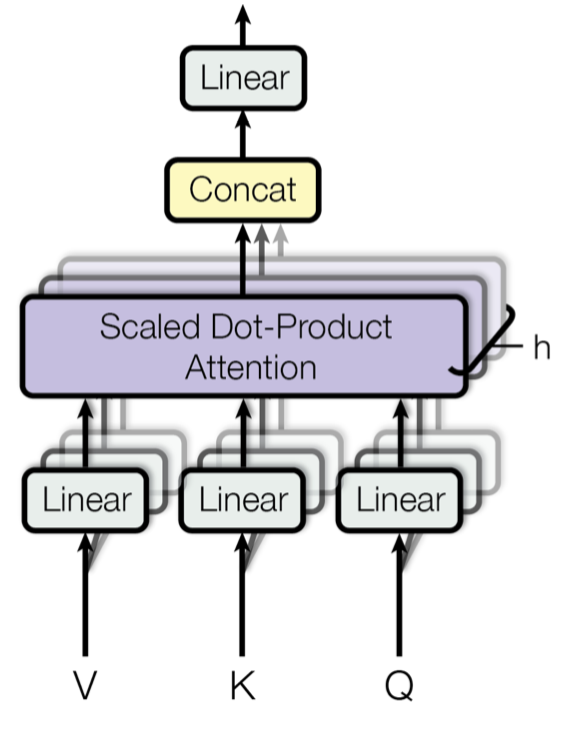
The multi-head self-attention module is a central component of Transformer. Instead of computing attention only once, the multi-head design partitions the inputs into smaller chunks and computes scaled dot-product attention in parallel within each subspace. The attention outputs from the different heads are then concatenated and passed through a linear transformation to produce the desired dimensionality.
Here, $[.;.]$ denotes concatenation. $\mathbf{W}^q_i, \mathbf{W}^k_i \in \mathbb{R}^{d \times d_k/h}, \mathbf{W}^v_i \in \mathbb{R}^{d \times d_v/h}$ are the weight matrices that project input embeddings of size $L \times d$ into the query, key, and value matrices. $\mathbf{W}^o \in \mathbb{R}^{d_v \times d}$ is the linear output projection. All of these weights are learned during training.
Transformer
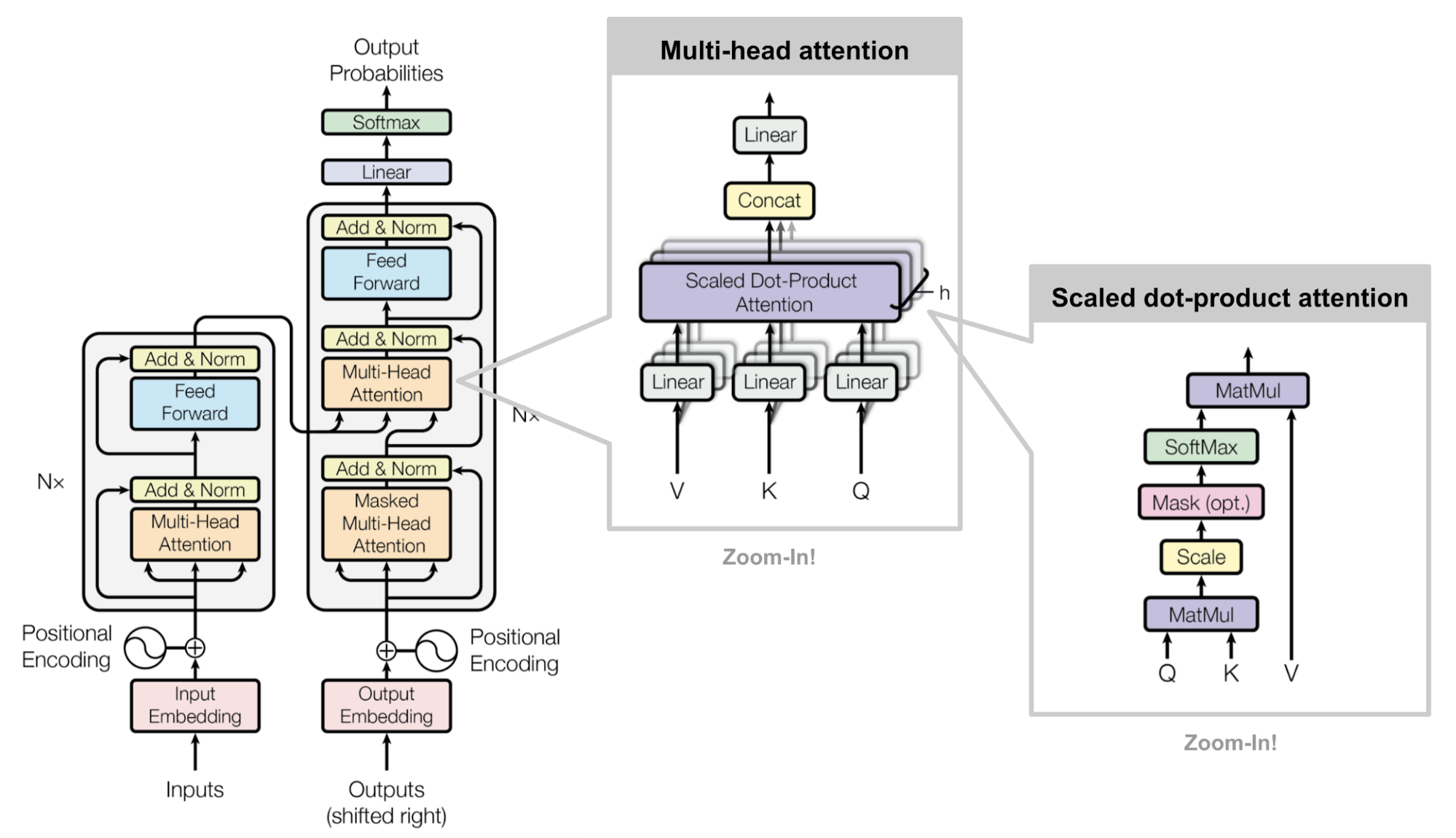
The Transformer model (referred to here as the “vanilla Transformer” to distinguish it from later enhanced variants; Vaswani, et al., 2017) uses an encoder-decoder architecture, a common design in many NMT models. Later work demonstrated that simplified Transformer variants can achieve excellent results in language modeling, such as encoder-only BERT and decoder-only GPT.
Encoder-Decoder Architecture
The encoder produces an attention-based representation with the ability to pinpoint specific information within a broad context. It is composed of a stack of 6 identical modules, each containing two submodules: a multi-head self-attention layer and a point-wise fully connected feed-forward network. “Point-wise” indicates that the same linear transformation (using shared weights) is applied independently to each element in the sequence. This is also equivalent to a convolutional layer with filter size 1. Each submodule includes a residual connection and layer normalization. All submodules emit outputs with the same dimensionality $d$.
The Transformer decoder retrieves information from the encoder’s representation. Its structure largely mirrors the encoder, except that each repeated module contains two multi-head attention submodules rather than one. The first of these multi-head attention submodules is masked to prevent positions from attending to future tokens.
Positional Encoding
Because self-attention is permutation-invariant, an explicit positional encoding is necessary to provide order information to the model. The positional encoding $\mathbf{P} \in \mathbb{R}^{L \times d}$ has the same dimensionality as the input embedding, allowing it to be added directly to the input. The vanilla Transformer explored two types of positional encodings:
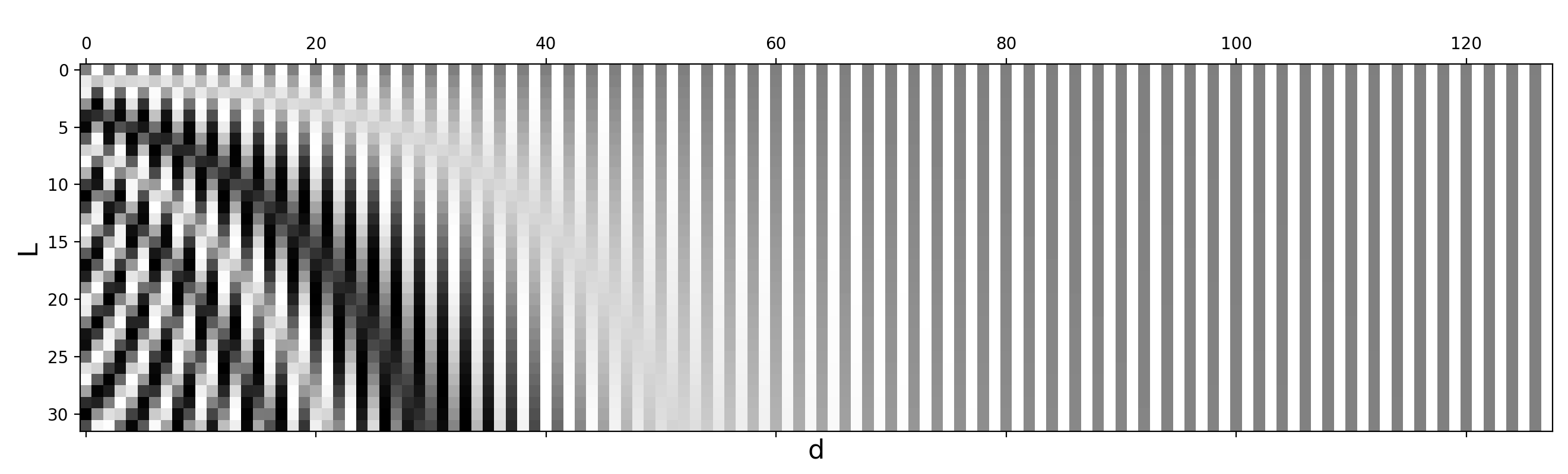
(1) Sinusoidal positional encoding is defined as follows, given token position $i=1,\dots,L$ and dimension $\delta=1,\dots,d$:
With this construction, each positional-encoding dimension corresponds to a sinusoid with a different wavelength, spanning from $2\pi$ to $10000 \cdot 2\pi$.
(2) Learned positional encoding assigns each element a learned column vector that encodes its absolute position (Gehring, et al. 2017).
Quick Follow-ups
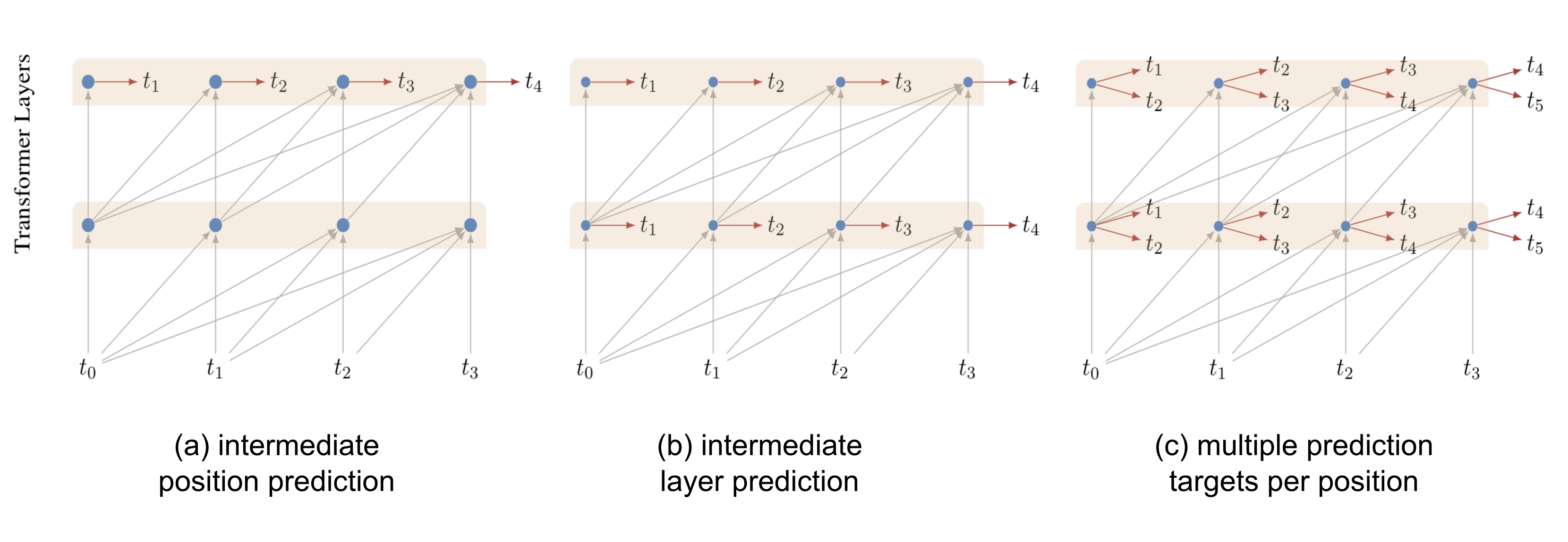
Building on the vanilla Transformer, Al-Rfou et al. (2018) introduced a collection of auxiliary losses to enable training a deep Transformer for character-level language modeling, achieving performance that surpassed LSTMs. Their approach uses several auxiliary tasks:
- Rather than generating only a single prediction at the end of the sequence, every intermediate position is also required to produce a correct prediction. This forces the model to learn to predict from smaller contexts (for example, the first few tokens at the start of a context window).
- Predictions are made from each intermediate Transformer layer as well. As training proceeds, lower layers are assigned progressively smaller weights in their contribution to the total loss.
- Each sequence position can predict multiple targets, meaning two or more predictions for future tokens.
Adaptive Computation Time (ACT)
Adaptive Computation Time (short for ACT; Graves, 2016) is a mechanism that dynamically determines how many computational steps are required in a recurrent neural network. distill.pub provides a helpful tutorial on ACT.
Consider an RNN model $\mathcal{R}$ defined by input weights $W_x$, a parametric state transition function $\mathcal{S}(.)$, output weights $W_y$, and an output bias $b_y$. Given an input sequence $(x_1, \dots, x_L)$, the output sequence $(y_1, \dots, y_L)$ is computed as:
ACT modifies this setup so that, for each input element, the model can execute a variable number of computation steps. Multiple internal steps produce a sequence of intermediate states $(s_t^1, \dots, s_t^{N(t)})$ and outputs $(y_t^1, \dots, y_t^{N(t)})$. These share the same state transition function $\mathcal{S}(.)$, as well as the same output weights $W_y$ and bias $b_y$:
where $\delta_{n,1}$ is a binary flag indicating whether the input step has advanced.
The number of steps $N(t)$ is determined by an additional sigmoidal halting unit $h$, with weight matrix $W_h$ and bias $b_h$. It outputs a halting probability $p_t^n$ at intermediate step $n$ for the $t$-th input element:
To make it possible to halt after just one step, ACT introduces a small constant $\epsilon$ (e.g. 0.01). Whenever the cumulative probability exceeds $1-\epsilon$, computation stops.
where $M$ is an upper bound on the number of intermediate steps allowed.
The final state and output are computed via mean-field updates:
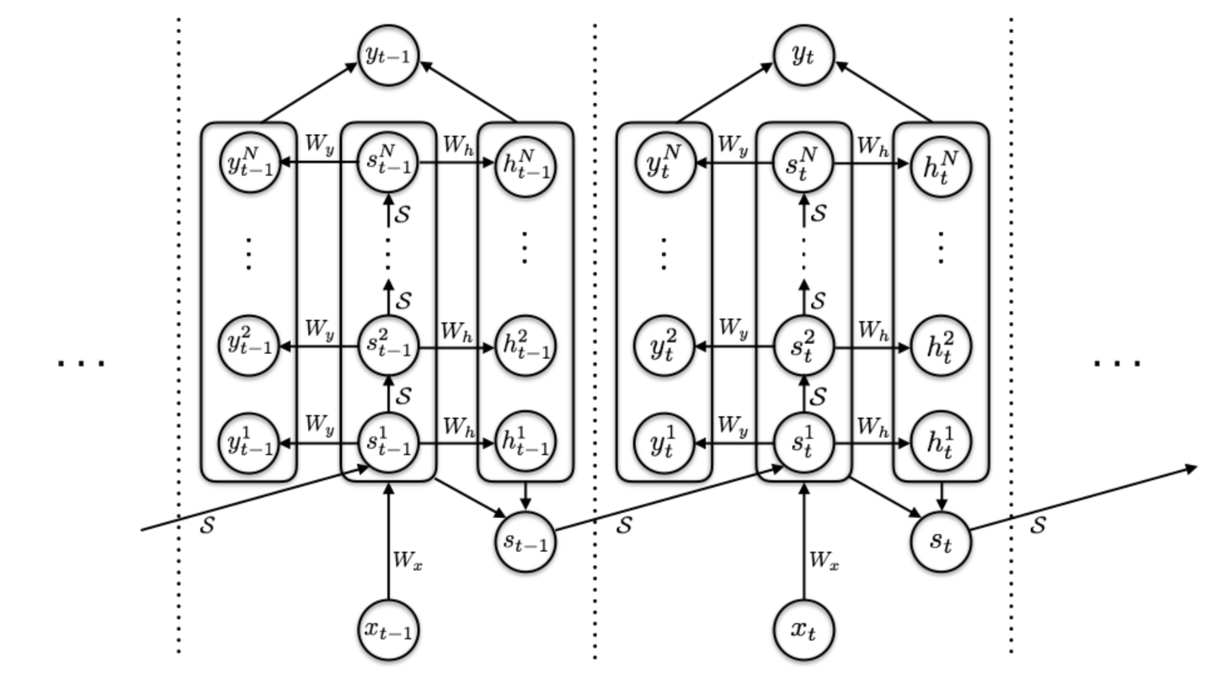
To discourage unnecessary computation on each input, ACT adds a ponder cost $\mathcal{P}(x) = \sum_{t=1}^L N(t) + R(t) $ in the loss function, encouraging fewer intermediate computation steps.
Improved Attention Span
Improving attention span aims to extend the usable context length in self-attention while keeping the mechanism efficient and flexible.
Longer Attention Span (Transformer-XL)
The vanilla Transformer has a fixed and limited attention span. In each update step, the model can attend only to elements within the same segment, and information cannot propagate across separate fixed-length segments.
This context segmentation leads to several problems:
- The model is unable to capture very long-term dependencies.
- Predicting the first few tokens in each segment is difficult because there is little to no preceding context.
- Evaluation is computationally expensive. Each time the segment shifts one position to the right, the new segment must be processed from scratch, even though many tokens overlap.
Transformer-XL (Dai et al., 2019; “XL” stands for “extra long”) addresses the context segmentation issue using two primary changes:
- Reusing hidden states across segments.
- Introducing a positional encoding scheme that works with state reuse.
Hidden State Reuse
Transformer-XL introduces recurrence between segments by continuously reusing hidden states from preceding segments.
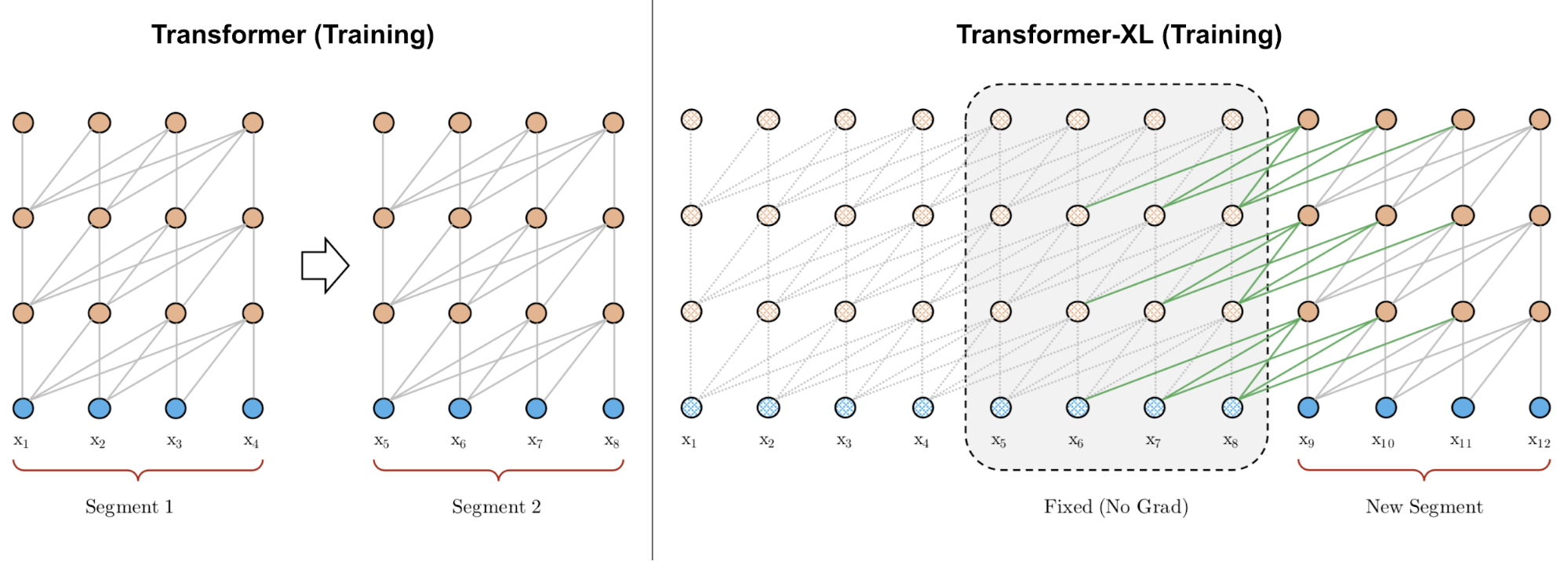
Let $\mathbf{h}_{\tau+1}^{(n)} \in \mathbb{R}^{L \times d}$ denote the hidden state at layer $n$ for segment $(\tau + 1)$. In addition to depending on the final-layer hidden state for the same segment $\mathbf{h}_{\tau+1}^{(n-1)}$, it also depends on the hidden state at the same layer from the previous segment $\mathbf{h}_{\tau}^{(n)}$. By injecting information from earlier hidden states, the model extends its effective attention span far into the past, across multiple segments.
Note that both the key and value are computed from the extended hidden state, while the query uses only the current-step hidden state. The concatenation operation $[. \circ .]$ is performed along the sequence-length dimension.
Relative Positional Encoding
To support this extended attention span, Transformer-XL proposes a new positional encoding approach. If vanilla Transformer style absolute positional encodings were used, then previous and current segments would receive identical encodings, which is not desirable.
To keep positional information consistent across segments, Transformer-XL instead encodes the relative position. In practice, it may be sufficient to know the offset between positions, that is, $i-j$, between a key vector $\mathbf{k}_{\tau, j}$ and its query $\mathbf{q}_{\tau, i}$.
If we ignore the scalar $1/\sqrt{d_k}$ and the softmax normalization term, but include positional encodings, the attention score between the query at position $i$ and the key at position $j$ can be written as:
Transformer-XL reparameterizes these four terms as:
- Replace $\mathbf{p}_j$ with relative positional encoding $\mathbf{r}_{i-j} \in \mathbf{R}^{d}$;
- Replace $\mathbf{p}_i\mathbf{W}^q$ with two trainable parameters $\mathbf{u}$ (for content) and $\mathbf{v}$ (for location) in two different terms;
- Split $\mathbf{W}^k$ into two matrices, $\mathbf{W}^k_E$ for content information and $\mathbf{W}^k_R$ for location information.
Adaptive Attention Span
A core strength of Transformer is its ability to capture long-term dependencies. Depending on the context, the model may sometimes prefer to attend farther back than at other times, and different attention heads may learn different attention patterns. If the attention span could adapt its effective length, attending farther into the past only when necessary, it could reduce both computation and memory requirements while supporting a longer maximum context length.
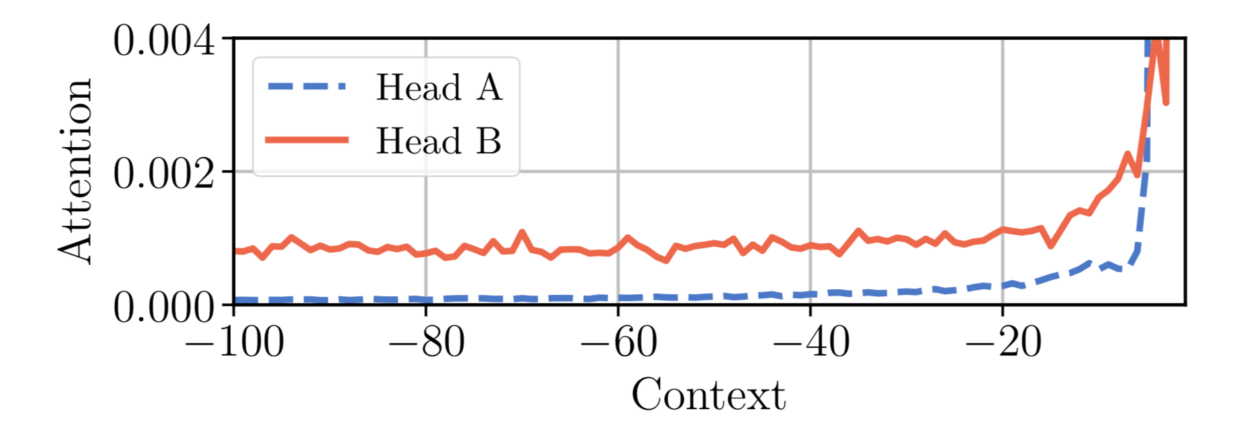
This is the motivation for Adaptive Attention Span. Sukhbaatar, et al., (2019) proposed a self-attention mechanism that aims to learn an optimal attention span. They hypothesized that different attention heads may allocate scores differently within the same context window (see Fig. 7), and therefore the optimal span should be trained separately for each head.
For the $i$-th token, we compute attention weights between this token and keys at positions $j \in S_i$, where $S_i$ defines the $i$-th token’s context window.
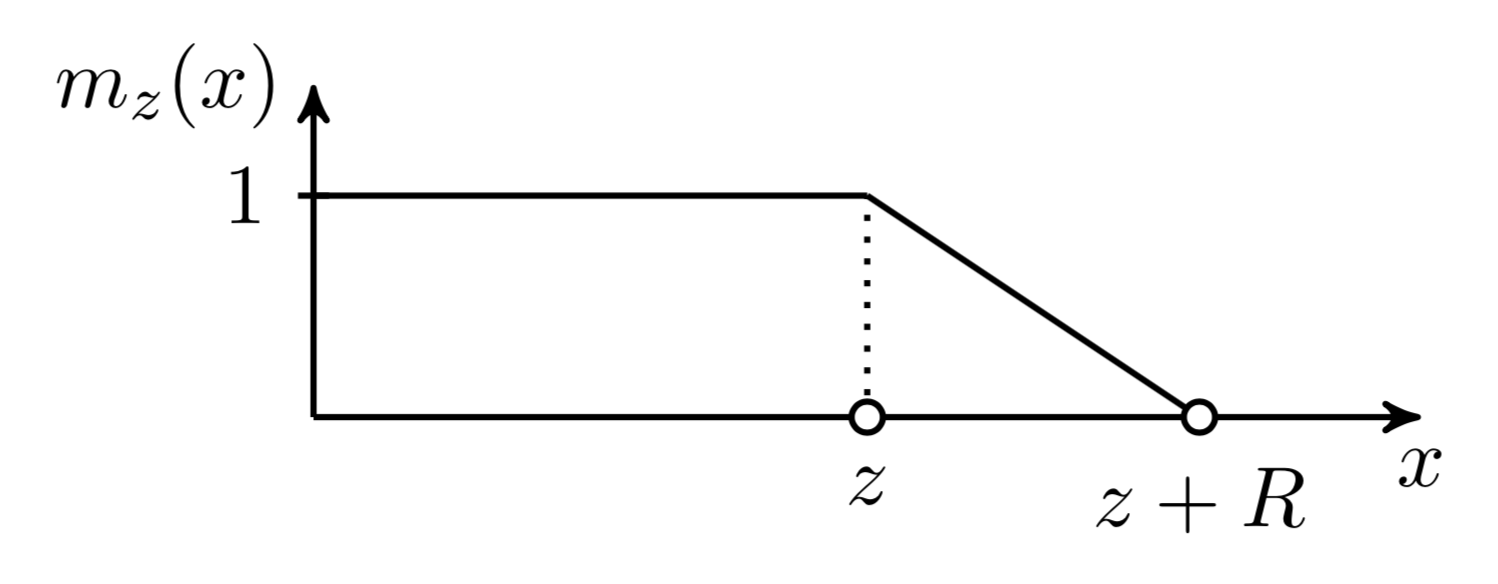
A soft mask function $m_z$ is introduced to control an effective, adjustable attention span. It maps the distance between query and key into a value in [0, 1]. $m_z$ is parameterized by $z \in [0, s]$, and $z$ is learned:
where $R$ is a hyper-parameter controlling the softness of $m_z$.
The soft mask function is applied to the softmax elements when computing attention weights:
In this equation, $z$ is differentiable, so it is trained jointly with the rest of the model. Parameters $z^{(i)}, i=1, \dots, h$ are learned separately per head. In addition, the loss includes an extra L1 penalty on $\sum_{i=1}^h z^{(i)}$.
Using Adaptive Computation Time, this method can be extended to produce a flexible attention span length that adapts dynamically to the current input. The span parameter $z_t$ of an attention head at time $t$ is modeled as a sigmoidal function, $z_t = S \sigma(\mathbf{v} \cdot \mathbf{x}_t +b)$, where the vector $\mathbf{v}$ and the bias scalar $b$ are learned jointly with the other parameters.
In experiments on Transformers with adaptive attention span, Sukhbaatar, et al. (2019) observed a general trend: lower layers typically do not require long attention spans, while a small number of attention heads in higher layers may adopt exceptionally long spans. Adaptive attention span also substantially reduces the number of FLOPS, particularly for large models with many attention layers and long context lengths.
Localized Attention Span (Image Transformer)
The original, and still most widely used, application of Transformer is language modeling. Text is a one-dimensional sequence with a clear chronological order, so the attention span grows linearly as context length increases.
However, when applying Transformer to images, the appropriate context scope and ordering are less obvious. Image Transformer (Parmer, et al 2018) adopts an image generation formulation analogous to sequence modeling within the Transformer framework. In addition, Image Transformer limits self-attention to local neighborhoods so the model can scale to process more images in parallel while keeping the likelihood loss tractable.
The encoder-decoder design is retained for image-conditioned generation:
- The encoder produces a contextualized representation of the source image for each pixel channel.
- The decoder generates the output image autoregressively, producing one channel per pixel at each time step.
Let the representation of the current pixel to be generated be the query $\mathbf{q}$. The representations at other positions used to compute $\mathbf{q}$ are key vectors $\mathbf{k}_1, \mathbf{k}_2, \dots$, and together they form a memory matrix $\mathbf{M}$. The scope $\mathbf{M}$ determines the context window for pixel query $\mathbf{q}$.
Image Transformer proposes two forms of localized $\mathbf{M}$, illustrated below.
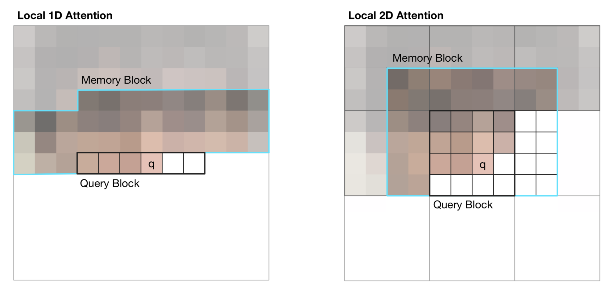
(1) 1D Local Attention: The input image is flattened using raster scanning order, from left to right and top to bottom. The resulting linearized image is partitioned into non-overlapping query blocks. The context window includes pixels within the same query block as $\mathbf{q}$, plus a fixed number of additional pixels generated prior to that query block.
(2) 2D Local Attention: The image is divided into multiple non-overlapping rectangular query blocks. A query pixel can attend to every other pixel within the same memory block. To ensure that the pixel in the top-left corner also receives a valid context window, the memory block is extended upward, to the left, and to the right by fixed amounts, respectively.
Less Time and Memory Cost
This section describes several Transformer modifications designed to reduce computation time and memory usage.
Sparse Attention Matrix Factorization (Sparse Transformers)
In the standard Transformer, computation and memory scale quadratically with sequence length, making it difficult to apply to very long sequences.
Sparse Transformer (Child et al., 2019) introduced factorized self-attention via sparse matrix factorization. This approach makes it feasible to train dense attention networks with hundreds of layers on sequences up to length 16,384, which would otherwise be infeasible on modern hardware.
Given an attention connectivity pattern $\mathcal{S} = \{S_1, \dots, S_n\}$, each $S_i$ records the set of key positions that the $i$-th query vector attends to.
Note that while the size of $S_i$ is not fixed, $a(\mathbf{x}_i, S_i)$ is always of size $d_v$, and thus $\text{Attend}(\mathbf{X}, \mathcal{S}) \in \mathbb{R}^{L \times d_v}$.
In anto-regressive models, one attention span is defined as $S_i = \{j: j \leq i\}$, because it allows each token to attend to all past positions.
In factorized self-attention, the set $S_i$ is decomposed into a tree of dependencies such that, for every pair of $(i, j)$ where $j \leq i$, there exists a path connecting $i$ back to $j$, and $i$ can attend to $j$ either directly or indirectly.
More precisely, the set $S_i$ is partitioned into $p$ non-overlapping subsets, where the $m$-th subset is denoted $A^{(m)}_i \subset S_i, m = 1,\dots, p$. Consequently, the path between output position $i$ and any $j$ has maximum length $p + 1$. For example, if $(j, a, b, c, \dots, i)$ is a path of indices between $i$ and $j$, then we would have $j \in A_a^{(1)}, a \in A_b^{(2)}, b \in A_c^{(3)}, \dots$, and so on.
Sparse Factorized Attention
Sparse Transformer proposed two types of fractorized attention. The concepts are easier to grasp using the 2D image examples shown in Fig. 10.
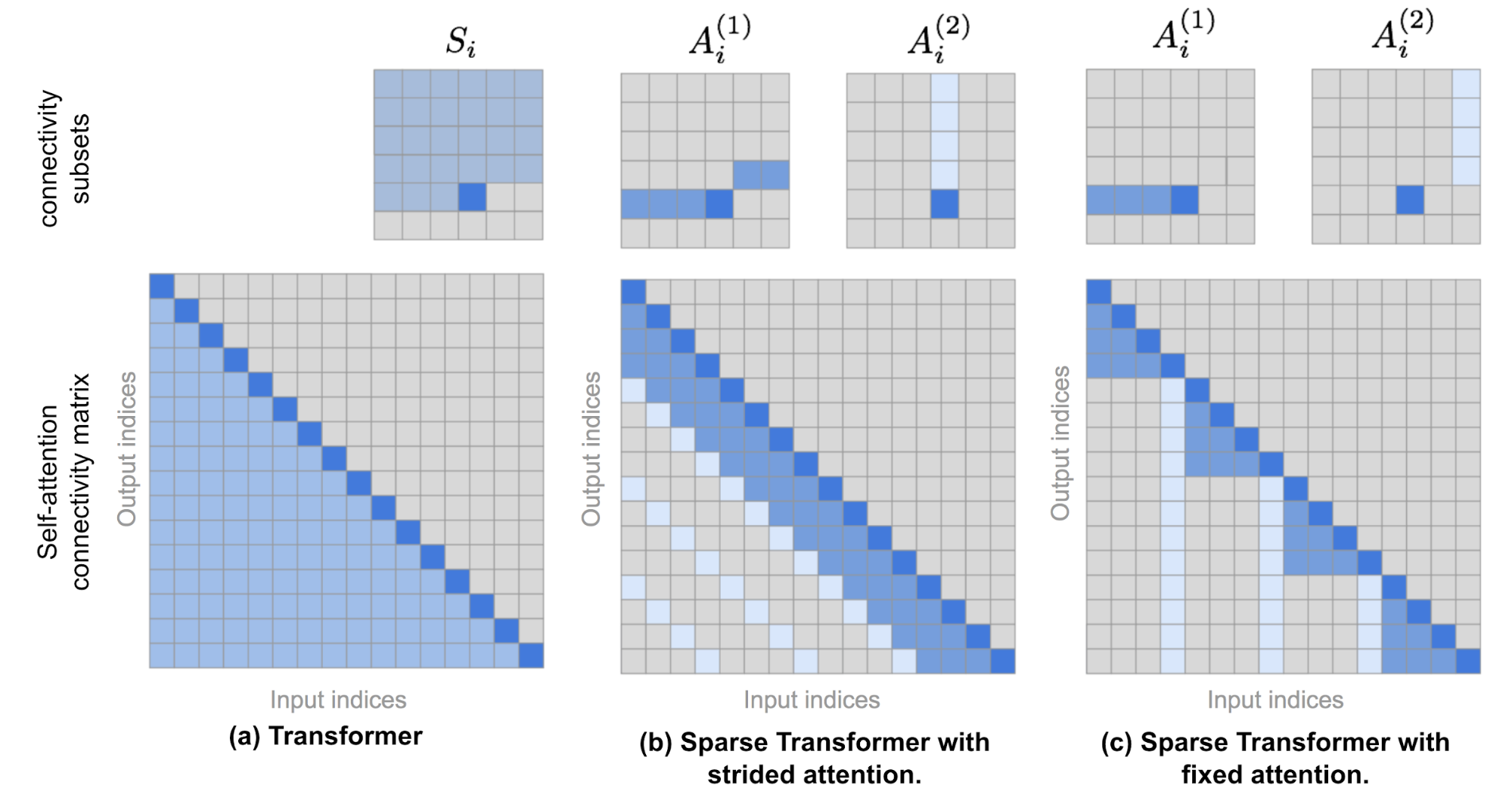
(1) Strided attention with stride $\ell \sim \sqrt{n}$. This pattern works well for image data because the structure aligns naturally with strides. In the image setting, each pixel attends to all previous $\ell$ pixels in raster-scan order (which naturally covers the full image width), and those pixels then attend to others in the same column (as defined by another attention connectivity subset).
(2) Fixed attention. A small set of tokens summarizes earlier locations and propagates that information to all future locations.
where $c$ is a hyperparameter. If $c=1$, it constrains the representation, because many positions then depend on only a few positions. The paper selected $c\in \{ 8, 16, 32 \}$ for $\ell \in \{ 128, 256 \}$.
Use Factorized Self-Attention in Transformer
There are three ways to incorporate sparse factorized attention patterns into the Transformer architecture:
- Assign one attention type per residual block and interleave them,
$\text{attention}(\mathbf{X}) = \text{Attend}(\mathbf{X}, A^{(n \mod p)}) \mathbf{W}^o$, where $n$ is the index of the current residual block. - Configure a single head to attend to the union of locations attended by all factorized heads,
$\text{attention}(\mathbf{X}) = \text{Attend}(\mathbf{X}, \cup_{m=1}^p A^{(m)}) \mathbf{W}^o $. - Use multi-head attention, but unlike the vanilla Transformer, each head may adopt a pattern from options 1 or 2. => This option often delivers the best performance.
Sparse Transformer also introduced several changes that enable training Transformers with up to hundreds of layers, including gradient checkpointing, recomputing attention & FF layers during the backward pass, mixed precision training, efficient block-sparse implementations, etc. For additional details, please refer to the paper.
Locality-Sensitive Hashing (Reformer)
The Reformer model (Kitaev, et al. 2020) proposed improvements intended to address the following pain points in Transformer:
- In a model with $N$ layers, memory usage is $N$-times larger than in a single-layer model, because activations must be stored for back-propagation.
- The intermediate FF layers are often very large.
- The attention matrix for sequences of length $L$ typically requires $O(L^2)$ in both memory and time.
Reformer introduced two primary changes:
- Replace dot-product attention with locality-sensitive hashing (LSH) attention, reducing complexity from $O(L^2)$ to $O(L\log L)$.
- Replace standard residual blocks with reversible residual layers, enabling activations to be stored only once during training instead of $N$ times (that is, proportional to the number of layers).
Locality-Sensitive Hashing Attention
In $\mathbf{Q} \mathbf{K}^\top$ part of the attention formula, only the largest elements matter, because after softmax, large values dominate the contribution. For each query $\mathbf{q}_i \in \mathbf{Q}$, we want to find row vectors in $\mathbf{K}$ that are closest to $\mathbf{q}_i$. To efficiently find nearest neighbors in high-dimensional space, Reformer integrates Locality-Sensitive Hashing (LSH) into its attention mechanism.
A hashing scheme $x \mapsto h(x)$ is locality-sensitive if it preserves distance information between data points, such that nearby vectors receive similar hashes, while far-apart vectors receive very different hashes. Reformer uses such a scheme: given a fixed random matrix $\mathbf{R} \in \mathbb{R}^{d \times b/2}$ (where $b$ is a hyperparam), the hash function is $h(x) = \arg\max([xR; −xR])$.
If we omit the scalar in self-attention and summarize the denominator into a normalizing term $Z(.)$, an normal attention output looks as follows: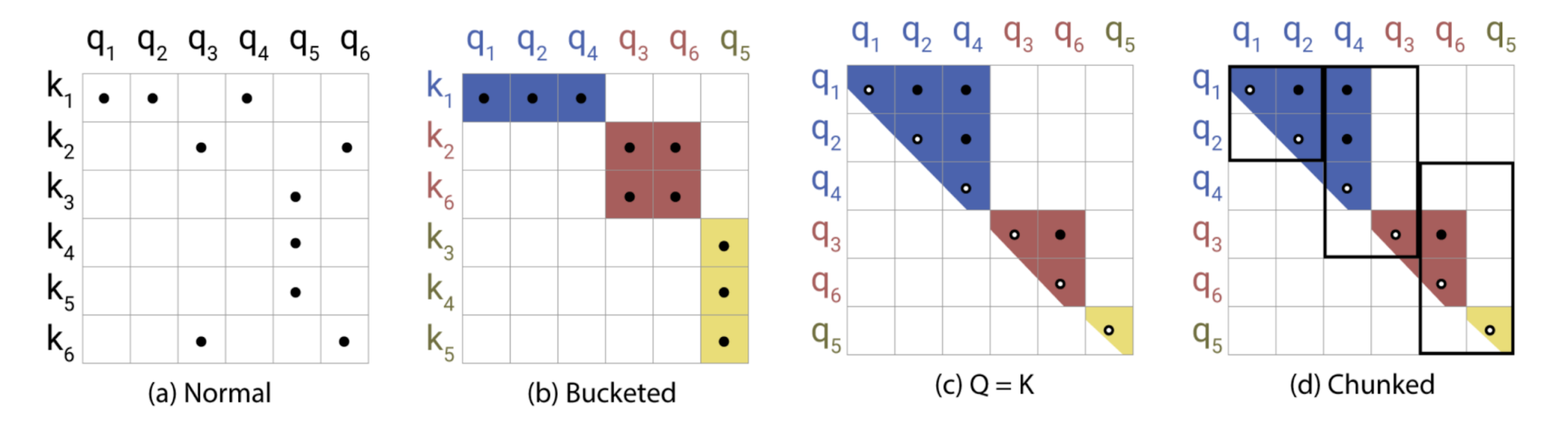
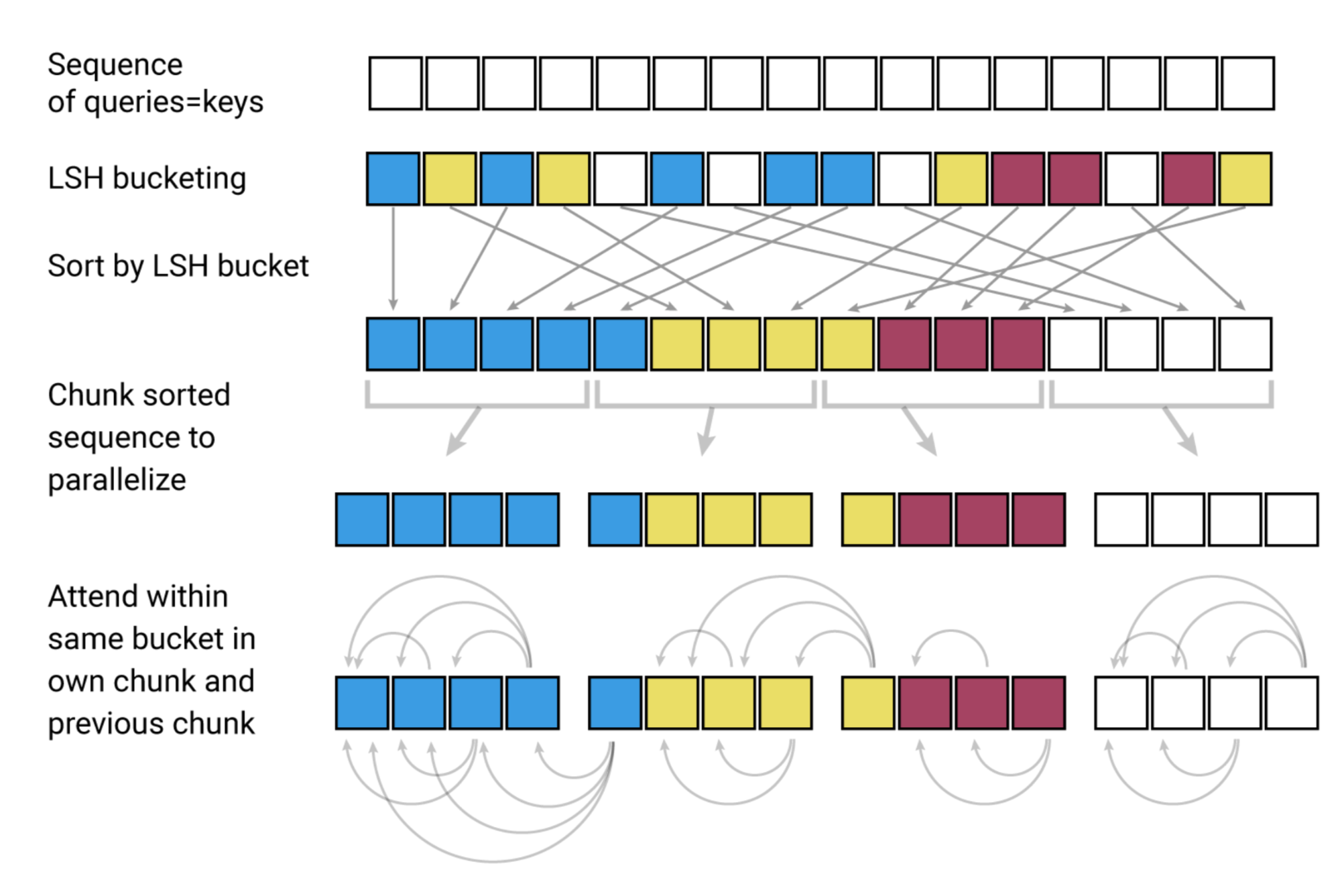
In LSH attention, a query can attend only to positions within the same hashing bucket, $S_i = \{j: h(\mathbf{q}_i) = h(\mathbf{k}_j)\}$. The method proceeds as follows, as illustrated in Fig. 11:
- (a) The full-attention matrix is often sparse.
- (b) With LSH, we can sort keys and queries so they align by hash bucket.
- (c) Set $\mathbf{Q} = \mathbf{K}$ (precisely $\mathbf{k}_j = \mathbf{q}_j / |\mathbf{q}_j|$) so that each bucket contains equal numbers of keys and queries, which simplifies batching. Notably, this “shared-QK” configuration does not affect Transformer performance.
- (d) Apply batching by grouping chunks of $m$ consecutive queries.
Reversible Residual Network
Another Reformer improvement is the use of reversible residual layers (Gomez et al. 2017). The goal of a reversible residual network is to construct an architecture in which activations at any layer can be reconstructed from the activations at the subsequent layer, using only model parameters. As a result, memory can be saved by recomputing activations during backpropagation rather than storing all intermediate activations.
Given a layer $x \mapsto y$, a standard residual layer computes $y = x + F(x)$. In contrast, a reversible layer splits both the input and output into pairs $(x_1, x_2) \mapsto (y_1, y_2)$ and then performs:
Reversal is straightforward:
Reformer applies this idea to Transformer by combining attention ($F$) and feed-forward layers ($G$) within a reversible network block:
Memory usage can be reduced further by chunking the feed-forward computation:
The resulting reversible Transformer does not need to store activations at every layer.
Make it Recurrent (Universal Transformer)
The Universal Transformer (Dehghani, et al. 2019) combines Transformer self-attention with the recurrent mechanism of RNNs, aiming to capture both the long-term global receptive field provided by Transformer and the learned inductive biases of RNNs.
Instead of running through a fixed number of layers, the Universal Transformer dynamically selects the number of steps using adaptive computation time. When the number of steps is fixed, a Universal Transformer is equivalent to a multi-layer Transformer with parameters shared across layers.
At a high level, the Universal Transformer can be interpreted as a recurrent function that learns a hidden-state representation for each token. The recurrence evolves in parallel across token positions, and information is exchanged between positions through self-attention.
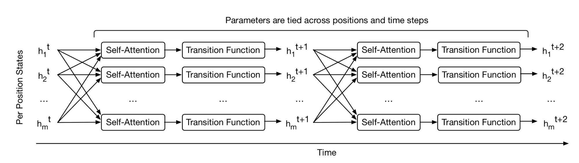
Given an input sequence of length $L$, the Universal Transformer iteratively updates the representation $\mathbf{H}^t \in \mathbb{R}^{L \times d}$ at step $t$ for an adjustable number of steps. At step 0, $\mathbf{H}^0$ is initialized to match the input embedding matrix. All positions are processed in parallel via multi-head self-attention and then passed through a recurrent transition function.
where $\text{Transition}(.)$ is either a separable convolution or a fully connected neural network composed of two position-wise (that is, applied to each row of $\mathbf{A}^t$ independently) affine transformations plus one ReLU.
The positional encoding $\mathbf{P}^t$ uses a sinusoidal position signal, augmented with an additional time dimension:
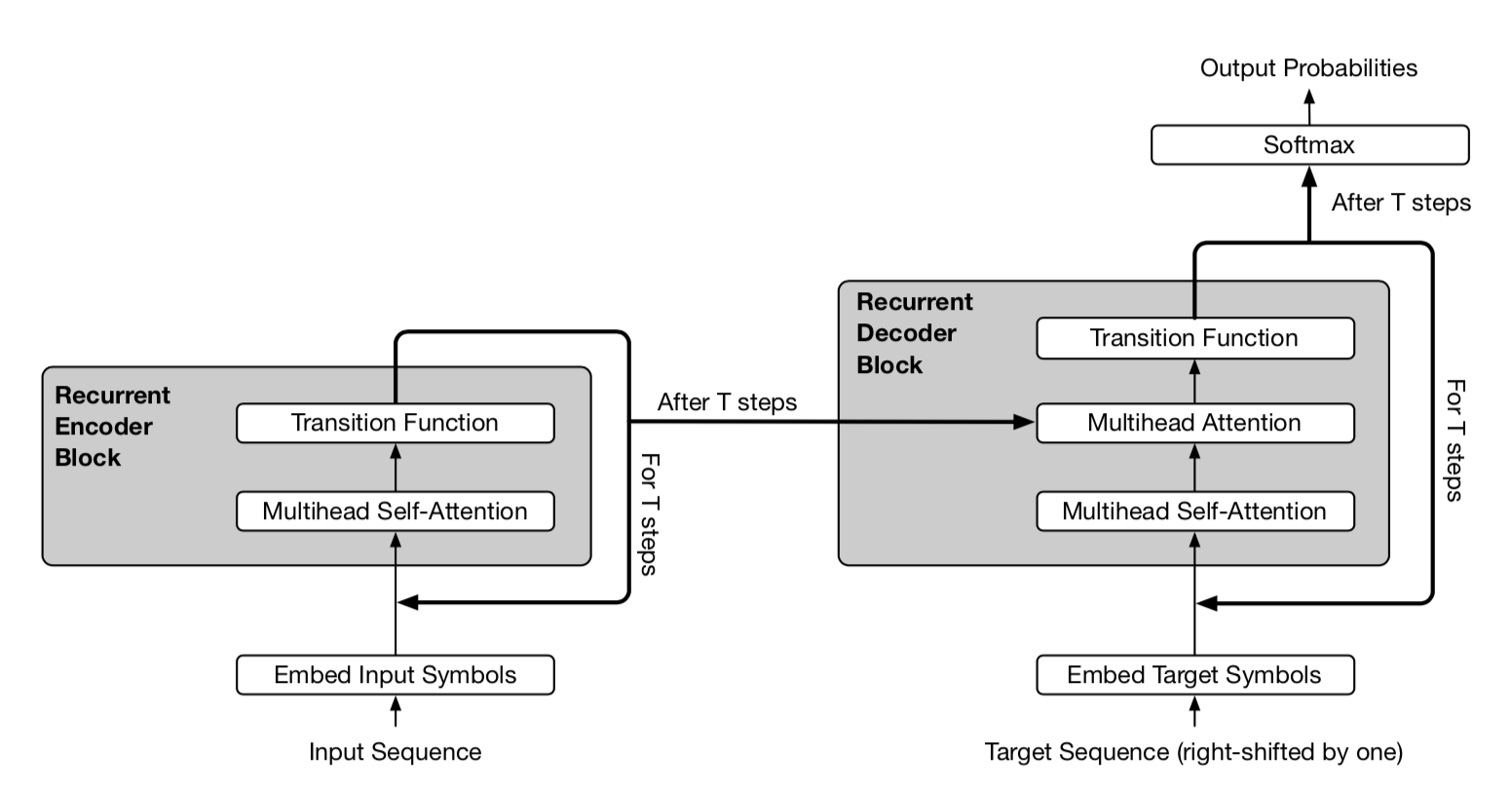
In the adaptive version of the Universal Transformer, the number of recurrent steps $T$ is determined dynamically by ACT. Each position is equipped with a dynamic ACT halting mechanism. Once a per-token recurrent block halts, it stops receiving further recurrent updates and instead copies its current value to the next step until all blocks halt or the model reaches a maximum step limit.
Stabilization for RL (GTrXL)
Self-attention avoids compressing the entire past into a fixed-size hidden state and is less prone to vanishing or exploding gradients than RNNs. Reinforcement learning tasks can certainly benefit from these properties. However, training Transformers can be difficult even in supervised settings, and it is even more challenging in RL. After all, stabilizing and training an LSTM agent alone can already be challenging.
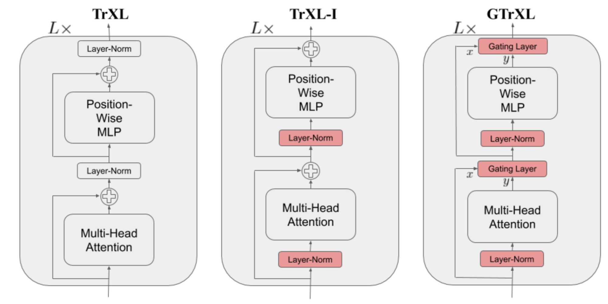
The Gated Transformer-XL (GTrXL; Parisotto, et al. 2019) is an attempt to apply Transformers to RL. GTrXL stabilized training with two modifications on top of Transformer-XL:
- Layer normalization is applied only to the input stream in a residual module, and not to the shortcut stream. A key benefit of this reordering is that it allows the original input to flow from the first layer to the last.
- The residual connection is replaced by a GRU-style (Gated Recurrent Unit; Chung et al., 2014) gating mechanism.
The parameters of the gating function are explicitly initialized to be close to an identity map, which is why the $b_g$ term appears. A $b_g > 0$ greatly improves learning speed.
Citation
Cited as:
Weng, Lilian. (Apr 2020). The transformer family. Lil’Log. https://lilianweng.github.io/posts/2020-04-07-the-transformer-family/.
Or
@article{weng2020transformer,
  title   = "The Transformer Family",
  author  = "Weng, Lilian",
  journal = "lilianweng.github.io",
  year    = "2020",
  month   = "Apr",
  url     = "https://lilianweng.github.io/posts/2020-04-07-the-transformer-family/"
}
Reference
[1] Ashish Vaswani, et al. “Attention is all you need.” NIPS 2017.
[2] Rami Al-Rfou, et al. “Character-level language modeling with deeper self-attention.” AAAI 2019.
[3] Olah & Carter, “Attention and Augmented Recurrent Neural Networks”, Distill, 2016.
[4] Sainbayar Sukhbaatar, et al. “Adaptive Attention Span in Transformers”. ACL 2019.
[5] Rewon Child, et al. “Generating Long Sequences with Sparse Transformers” arXiv:1904.10509 (2019).
[6] Nikita Kitaev, et al. “Reformer: The Efficient Transformer” ICLR 2020.
[7] Alex Graves. (“Adaptive Computation Time for Recurrent Neural Networks”)[https://arxiv.org/abs/1603.08983]
[8] Niki Parmar, et al. “Image Transformer” ICML 2018.
[9] Zihang Dai, et al. “Transformer-XL: Attentive Language Models Beyond a Fixed-Length Context.” ACL 2019.
[10] Aidan N. Gomez, et al. “The Reversible Residual Network: Backpropagation Without Storing Activations” NIPS 2017.
[11] Mostafa Dehghani, et al. “Universal Transformers” ICLR 2019.
[12] Emilio Parisotto, et al. “Stabilizing Transformers for Reinforcement Learning” arXiv:1910.06764 (2019).