Neural Architecture Search
Even though many of today’s most widely used and successful model architectures are crafted by human experts, this does not imply that the full space of possible network architectures has been thoroughly explored or that we have already converged on the best choice. We are more likely to identify an optimal solution by using a systematic, automated approach to discover and learn high-performance model architectures.
· 32 min read · Curated and presented by Arthur Sedek
Although many widely used and highly successful architectures are designed by human experts, that does not imply we have exhaustively explored the full architecture space or identified the optimal option. A more systematic and automated approach to learning high-performance architectures increases the likelihood of finding an optimal solution.
Automatically learning and evolving network topologies is not a new concept (Stanley & Miikkulainen, 2002). In recent years, the pioneering work by Zoph & Le 2017 and Baker et al. 2017 has drawn substantial attention to Neural Architecture Search (NAS), and it has led to many ideas for more effective, faster, and more resource-efficient NAS methods.
When I began studying NAS, I found the survey by Elsken, et al 2019 particularly helpful. They describe NAS as a system with three major components, which is a clean and concise framing that is also widely adopted across NAS papers.
- Search space: The NAS search space specifies a set of operations (e.g. convolution, fully-connected, pooling) and the permissible ways to connect them to form valid network architectures. Designing the search space typically requires human expertise and, inevitably, introduces human biases.
- Search algorithm: A NAS search algorithm samples a population of candidate architectures. It uses child model performance metrics as rewards (e.g. high accuracy, low latency) and optimizes to produce high-performing architecture candidates.
- Evaluation strategy: We must measure, estimate, or predict the performance of many proposed child models to provide feedback for the search algorithm. Candidate evaluation can be very expensive, and many methods have been proposed to reduce time or computational costs.
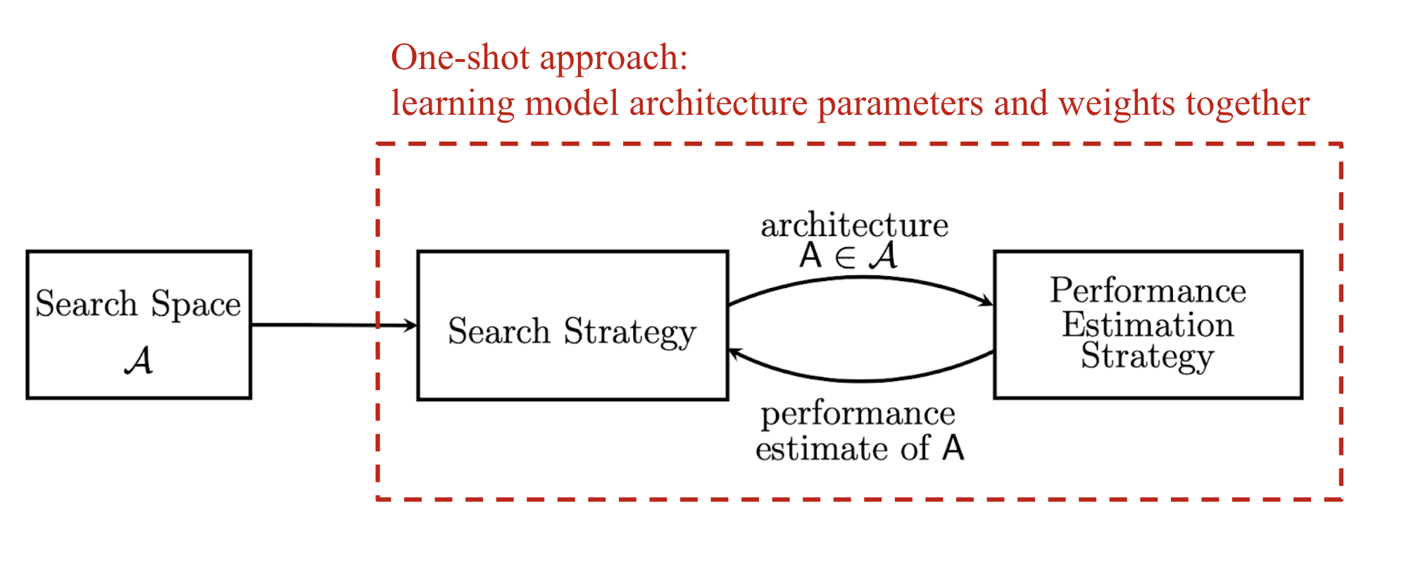
Search Space
The NAS search space defines a set of fundamental network operations and specifies how these operations may be connected to construct valid architectures.
Sequential Layer-wise Operations
The most straightforward way to define an architecture search space is to represent network topologies, whether CNN or RNN, as a list of sequential layer-wise operations, as in the early work of Zoph & Le 2017 and Baker et al. 2017. Serializing a network representation requires substantial expert knowledge because each operation has its own layer-specific parameters, and these associations must be hardcoded. For example, after predicting a conv op, the model must output kernel size, stride size, and so on. Similarly, after predicting an FC op, the next prediction must specify the number of units.
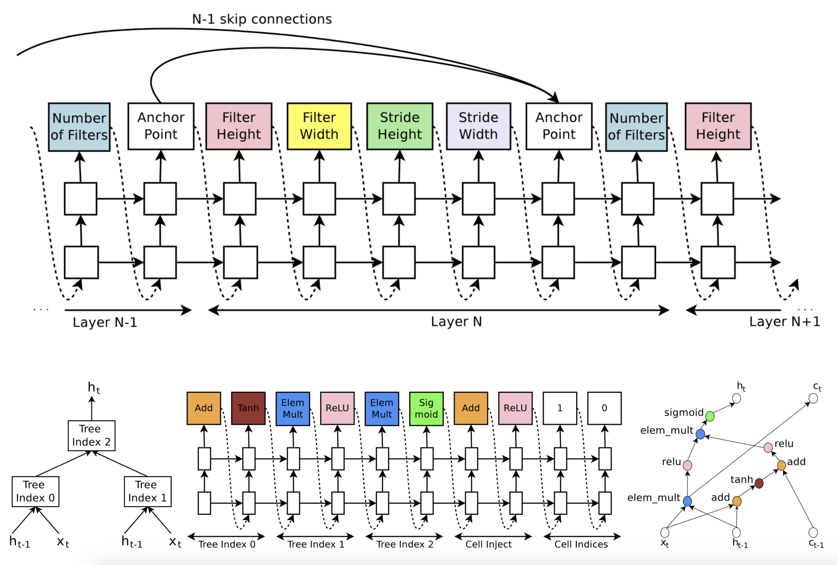
To ensure the generated architecture is valid, extra rules may be required (Zoph & Le 2017):
- If a layer is not connected to any input layer then it is used as the input layer;
- At the final layer, take all layer outputs that have not been connected and concatenate them;
- If one layer has many input layers, then all input layers are concatenated in the depth dimension;
- If input layers to be concatenated have different sizes, we pad the small layers with zeros so that the concatenated layers have the same sizes.
Skip connections can also be predicted, using an attention-style mechanism. At layer $i$, an anchor point is added with $i−1$ content-based sigmoids to indicate which previous layers should be connected. Each sigmoid takes as input the hidden states of the current node $h_i$ and $i-1$ previous nodes $h_j, j=1, \dots, i-1$.
While the sequential search space is highly expressive, it is also extremely large, and exhaustively exploring it requires substantial computational resources. In the experiments by Zoph & Le 2017, they ran 800 GPUs in parallel for 28 days, and Baker et al. 2017 constrained the search space to include at most 2 FC layers.
Cell-based Representation
Motivated by the repeated-module design used in successful vision architectures (e.g. Inception, ResNet), the NASNet search space (Zoph et al. 2018) defines a convolutional network as a single cell repeated multiple times, where each cell contains several operations predicted by the NAS algorithm. A well-designed cell module supports transfer across datasets, and the model size can be scaled down or up by adjusting the number of cell repeats.
More precisely, the NASNet search space learns two types of cells for network construction:
- Normal Cell: The input and output feature maps have the same dimension.
- Reduction Cell: The output feature map has its width and height reduced by half.
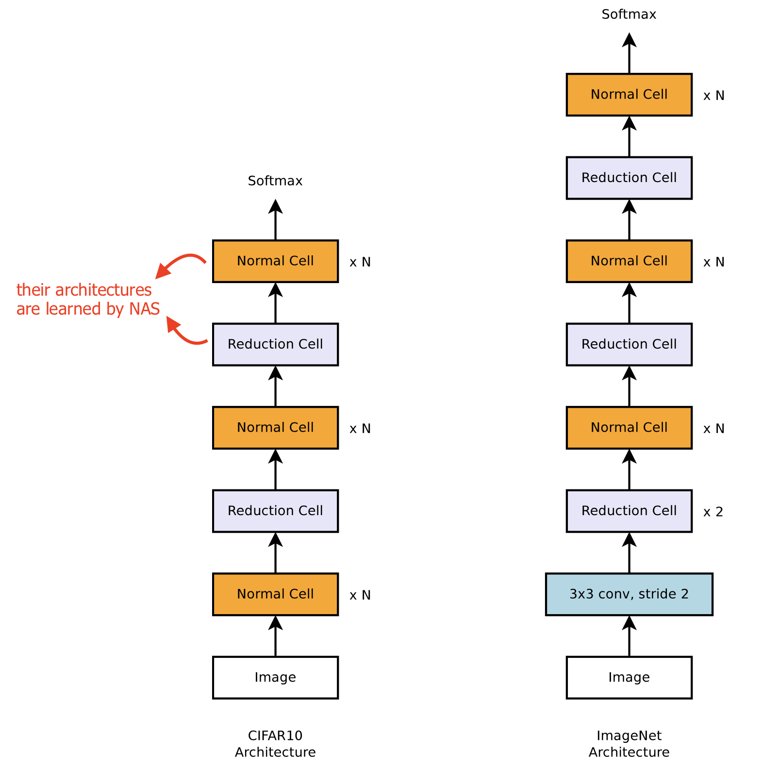
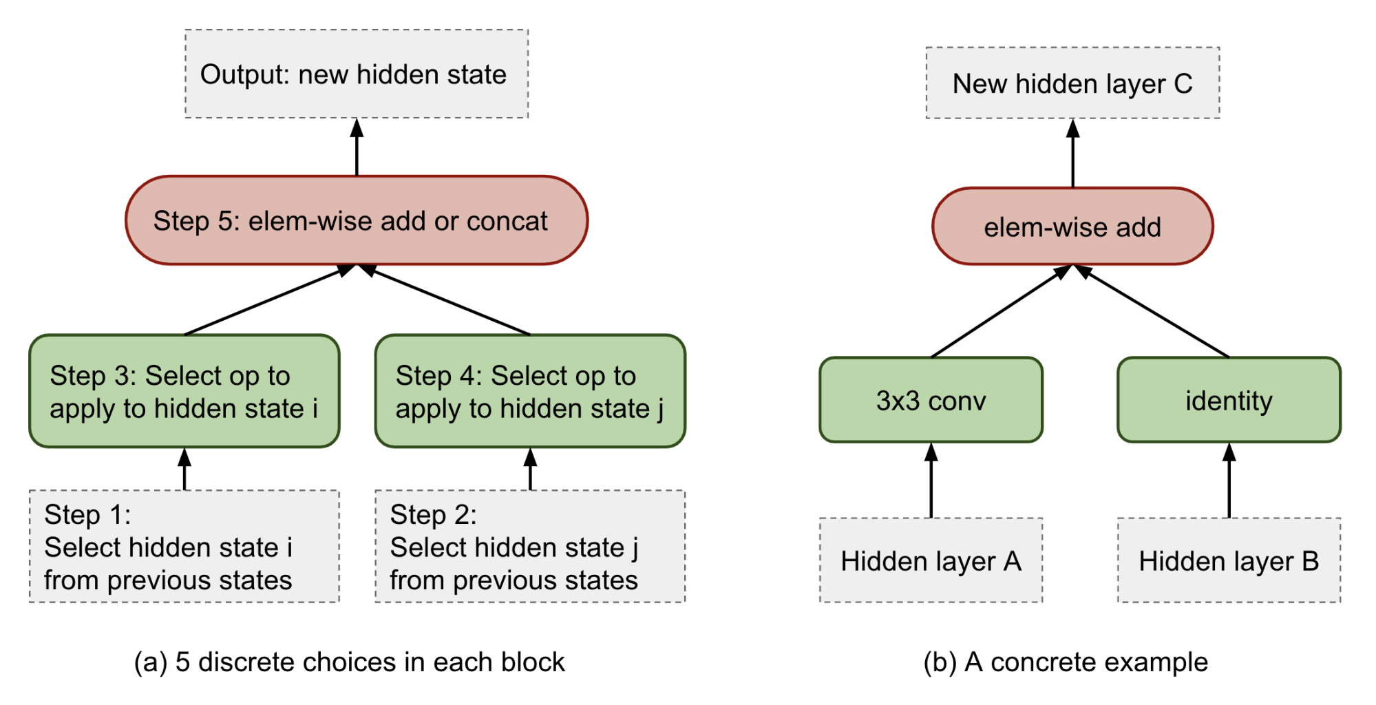
For each cell, predictions are organized into $B$ blocks ($B=5$ in the NASNet paper). Each block consists of five prediction steps produced by five distinct softmax classifiers, each corresponding to a discrete choice among the block elements. Note that the NASNet search space does not include residual connections between cells, and the model learns skip connections only within blocks.
During the experiments, they found that a modified version of DropPath, called ScheduledDropPath, significantly improves NASNet performance. DropPath stochastically drops paths (that is, edges with operations attached in NASNet) using a fixed probability. ScheduledDropPath applies DropPath with a linearly increasing path-drop probability over training.
Elsken, et al (2019) highlight three key advantages of the NASNet search space:
- The search space size is reduced drastically;
- The motif-based architecture can be more easily transferred to different datasets.
- It provides strong evidence for a useful design pattern in architecture engineering, namely repeatedly stacking modules. For example, strong CNNs can be built by stacking residual blocks, and strong Transformers can be built by stacking multi-headed attention blocks.
Hierarchical Structure
To capitalize on already discovered and well-designed network motifs, the NAS search space can be constrained to a hierarchical structure, as in Hierarchical NAS (HNAS; (Liu et al 2017)). It begins with a small set of primitives, including individual operations such as convolution, pooling, identity, and others. Small sub-graphs (or “motifs”) composed of primitive operations are then used recursively to form higher-level computation graphs.
A computation motif at level $\ell=1, \dots, L$ can be represented by $(G^{(\ell)}, \mathcal{O}^{(\ell)})$, where:
- $\mathcal{O}^{(\ell)}$ is a set of operations, $\mathcal{O}^{(\ell)} = \{ o^{(\ell)}_1, o^{(\ell)}_2, \dots \}$
- $G^{(\ell)}$ is an adjacency matrix, where the entry $G_{ij}=k$ indicates that operation $o^{(\ell)}_k$ is placed between node $i$ and $j$. The node indices follow topological ordering in DAG, where the index $1$ is the source and the maximal index is the sink node.
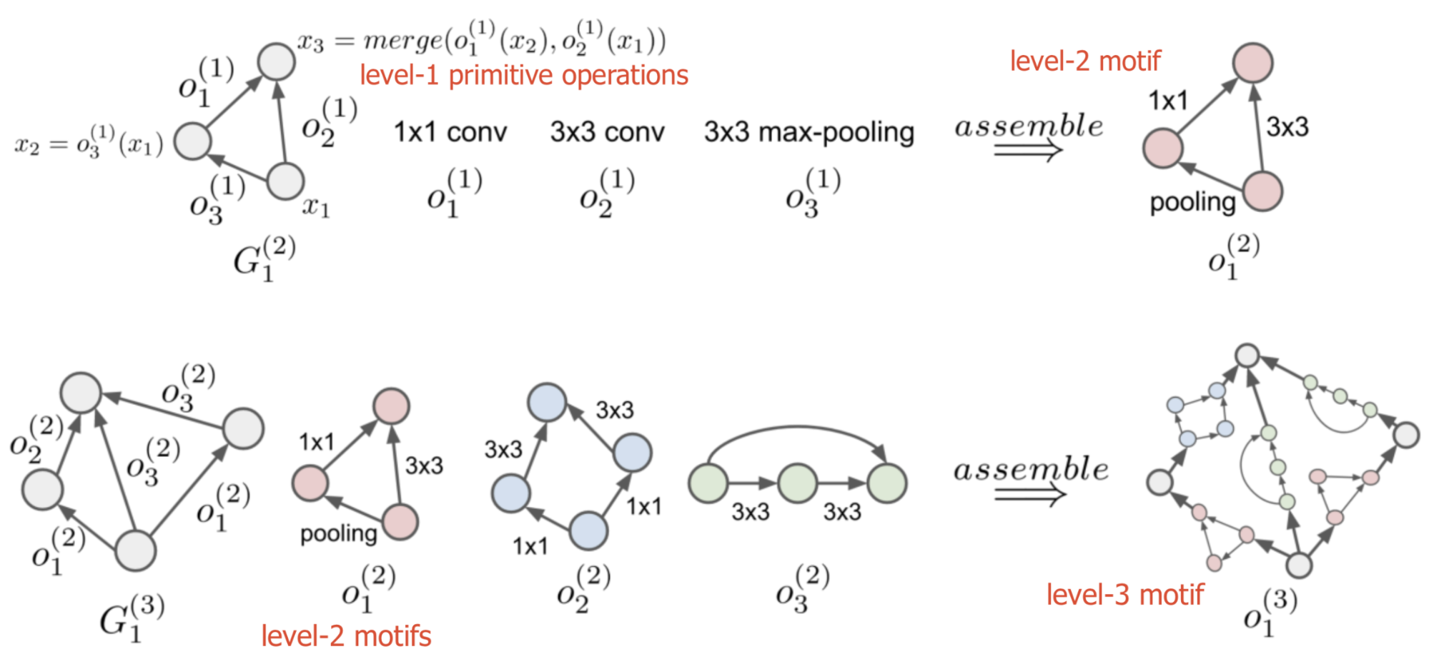
To construct a network under this hierarchical structure, we start from the lowest level $\ell=1$ and recursively define the $m$-th motif operation at level $\ell$ as:
A hierarchical representation becomes $\Big( \big\{ \{ G_m^{(\ell)} \}_{m=1}^{M_\ell} \big\}_{\ell=2}^L, \mathcal{O}^{(1)} \Big), \forall \ell=2, \dots, L$, where $\mathcal{O}^{(1)}$ contains a set of primitive operations.
The $\text{assemble}()$ process is equivalent to computing the feature map of node $i$ sequentially by aggregating the feature maps of all predecessor nodes $j$, following the topological ordering:
where $\text{merge}[]$ is implemented as depth-wise concatenation in the paper.
As with NASNet, the experiments in Liu et al (2017) focus on discovering strong cell architectures within a predefined “macro” structure built from repeated modules. They demonstrate that even simple search approaches (e.g. random search or evolutionary algorithms) can become substantially more effective when paired with well-designed search spaces.
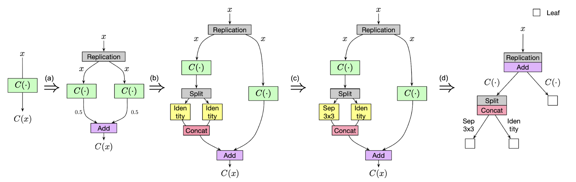
Cai et al (2018b) propose a tree-structured search space based on path-level network transformation. Each node in the tree defines an allocation scheme for splitting inputs among child nodes and a merge scheme for combining results from child nodes. Path-level network transformation enables replacing a single layer with a multi-branch motif when the corresponding merge scheme is add or concat.
Memory-bank Representation
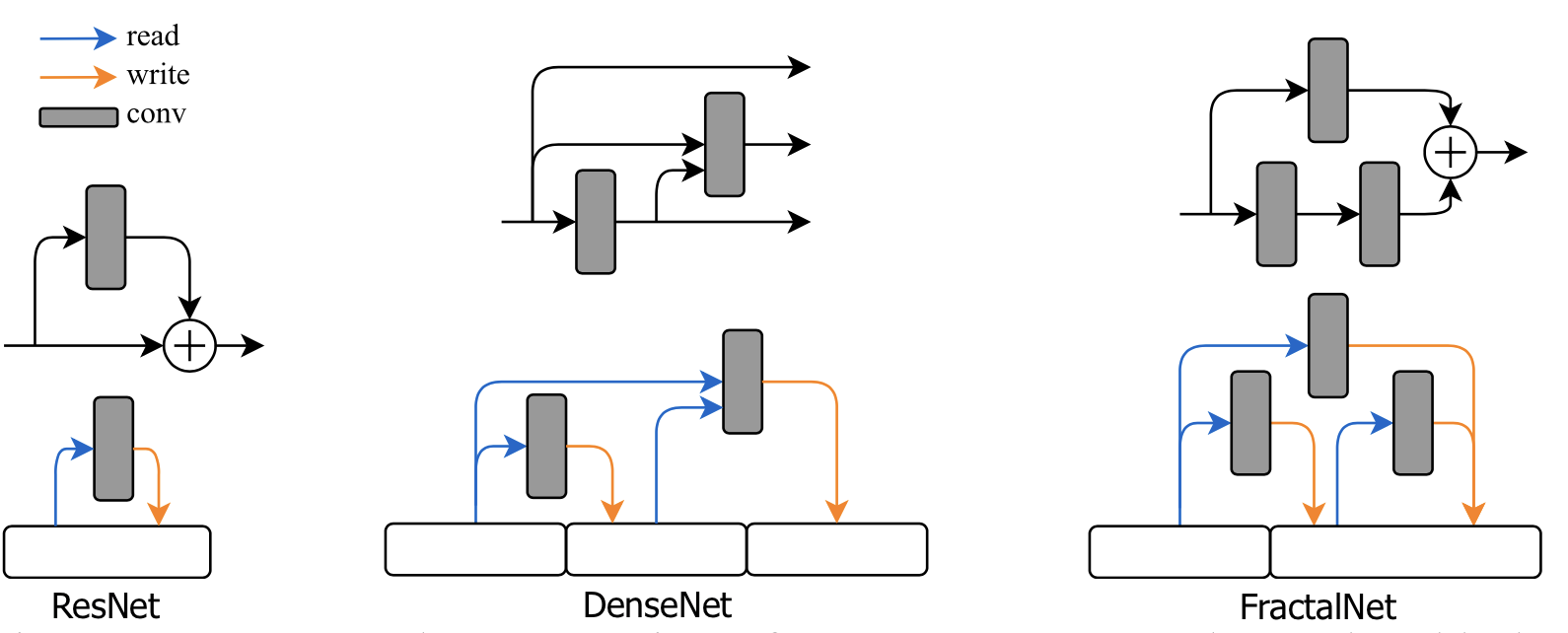
Brock et al. (2017) propose a memory-bank representation for feed-forward networks in SMASH. Rather than describing the model as a graph of operations, they treat a neural network as a system of multiple memory blocks with read and write capabilities. Each layer operation is designed to: (1) read from a subset of memory blocks; (2) compute results; and (3) write the results to another subset of blocks. For example, in a sequential model, a single memory block would be read and overwritten repeatedly.
Search Algorithms
NAS search algorithms sample a population of child networks. They receive child-model performance metrics as rewards and learn to propose high-performing architecture candidates. You may notice many similarities to the field of hyperparameter search.
Random Search
Random search is the simplest baseline. It samples a valid architecture candidate from the search space at random, and it does not involve a learned model. Random search has been shown to be effective for hyperparameter search (Bergstra & Bengio 2012). With a well-designed search space, random search can be a surprisingly difficult baseline to outperform.
Reinforcement Learning
The original NAS design (Zoph & Le 2017) uses an RL-based controller to propose child architectures for evaluation. The controller is implemented as an RNN that outputs a variable-length sequence of tokens used to configure a network architecture.
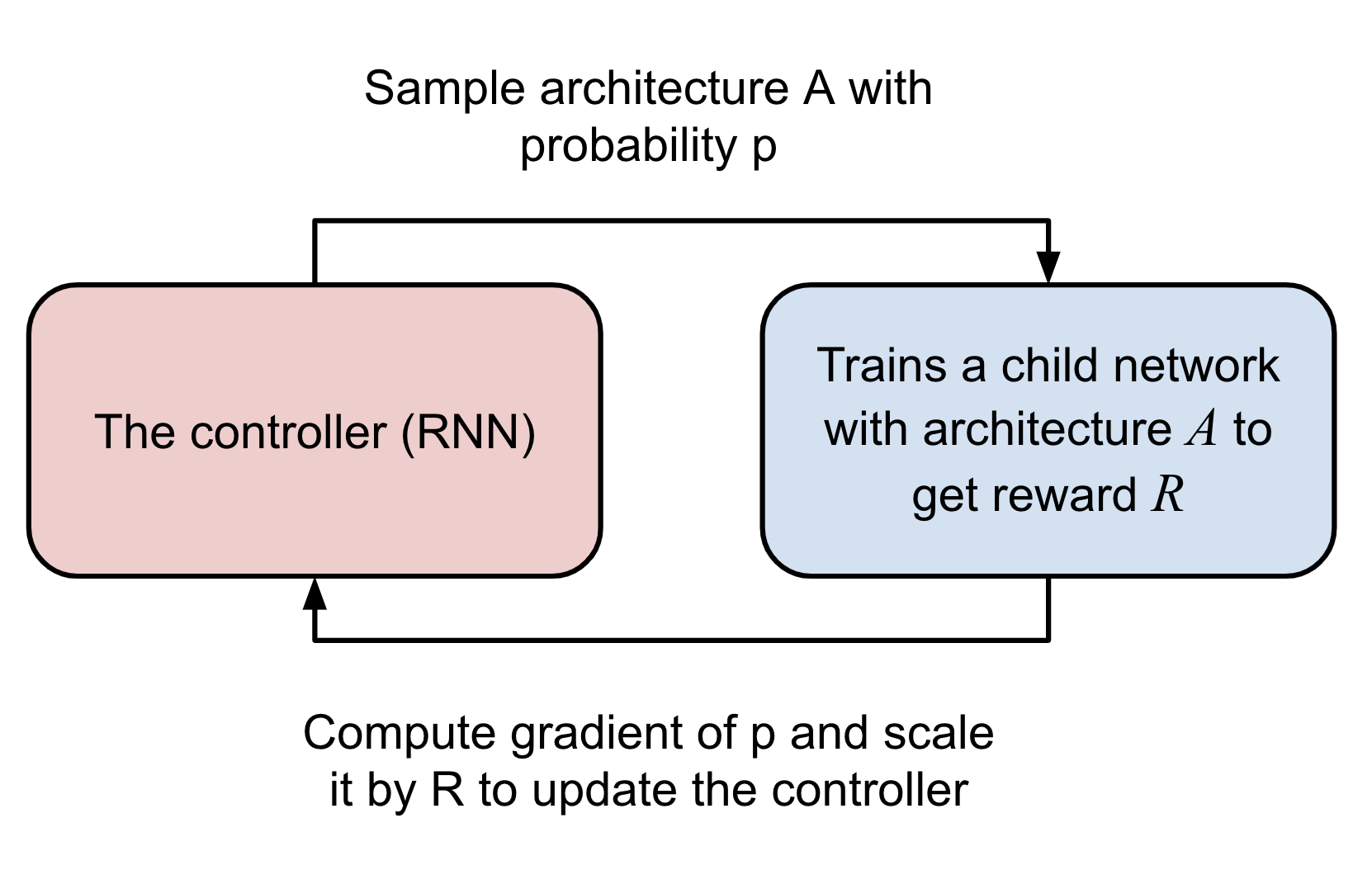
The controller is trained as an RL task using REINFORCE.
- Action space: The action space consists of the tokens predicted by the controller that define a child network (see the section above). The controller outputs the action $a_{1:T}$, where $T$ is the total number of tokens.
- Reward: The reward for training the controller is the accuracy a child network achieves at convergence, $R$.
- Loss: NAS optimizes the controller parameters $\theta$ using a REINFORCE loss. The goal is to maximize the expected reward (high accuracy) using the gradient below. A key advantage of policy gradients in this setting is that they remain applicable even when the reward is non-differentiable.
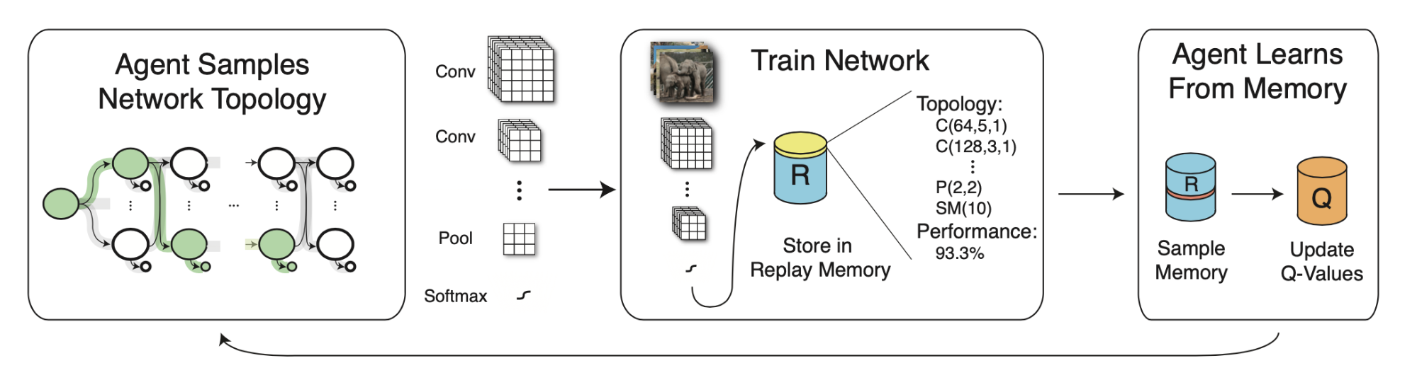
MetaQNN (Baker et al. 2017) trains an agent to choose CNN layers sequentially using Q-learning with an $\epsilon$-greedy exploration strategy and experience replay. The reward is also validation accuracy.
Here, a state $s_t$ is a tuple consisting of the layer operation and its related parameters. An action $a$ determines the connectivity between operations. The Q-value is proportional to the confidence that connecting two operations will lead to high accuracy.
Evolutionary Algorithms
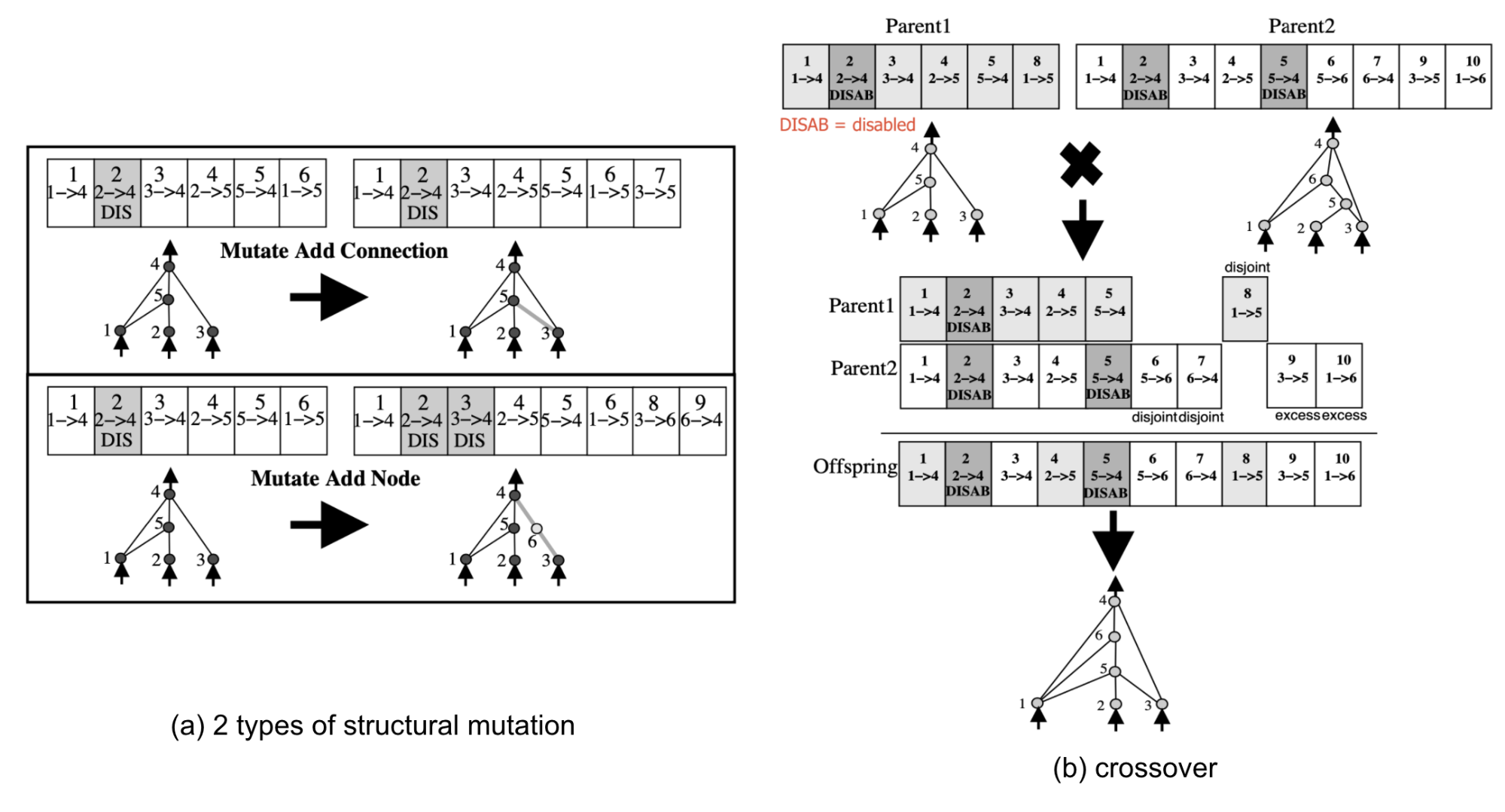
NEAT (short for NeuroEvolution of Augmenting Topologies) is a method for evolving neural network topologies with a genetic algorithm (GA), proposed by Stanley & Miikkulainen in 2002. NEAT evolves both connection weights and network topology jointly. Each gene encodes the complete information needed to configure a network, including node weights and edges. The population grows through mutations of both weights and connections, as well as crossovers between two parent genes. For more on neuroevolution, see the in-depth survey by Stanley et al. (2019).
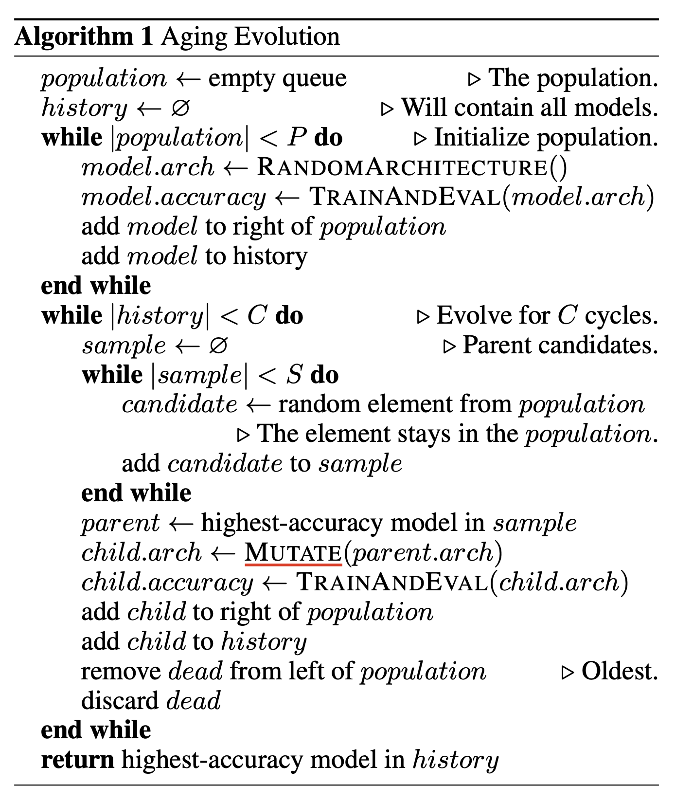
Real et al. (2018) use evolutionary algorithms (EA) to search for high-performing architectures in AmoebaNet. They apply tournament selection, where each iteration selects the best candidate from a random subset of samples and inserts its mutated offspring back into the population. When the tournament size is $1$, this becomes equivalent to random selection.
AmoebaNet modifies tournament selection to prefer younger genotypes and to always discard the oldest models in each cycle. This method, called aging evolution, encourages broader exploration of the search space rather than prematurely focusing on strong-performing models.
Specifically, in each cycle of tournament selection with aging regularization (See Figure 11):
- Sample $S$ models from the population, and choose the one with the highest accuracy as the parent.
- Create a child model by mutating the parent.
- Train and evaluate the child model, then add it back into the population.
- Remove the oldest model from the population.
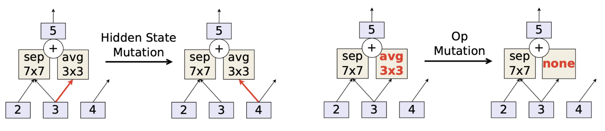
They apply two mutation types:
- Hidden state mutation: Randomly select a pairwise combination and rewire a random end, ensuring the resulting graph contains no loops.
- Operation mutation: Randomly replace an existing operation with a randomly chosen alternative.
In their experiments, EA and RL achieve comparable final validation accuracy, but EA provides better anytime performance and can discover smaller models. However, using EA for NAS remains computationally expensive, as each experiment took 7 days with 450 GPUs.
HNAS (Liu et al 2017) also uses evolutionary algorithms (original tournament selection) as its search strategy. In the hierarchical structure search space, each edge corresponds to an operation. Accordingly, genotype mutation in their experiments is performed by replacing a random edge with a different operation. The replacement set includes a none op, enabling edges to be altered, removed, or added. The initial genotype set is created by applying many random mutations to “trivial” motifs (all identity mappings).
Progressive Decision Process
Building a model architecture is inherently sequential, and every additional operator or layer increases complexity. If we encourage the search procedure to begin with simpler models and gradually evolve toward more complex architectures, this effectively introduces a “curriculum” into the search model’s learning process.
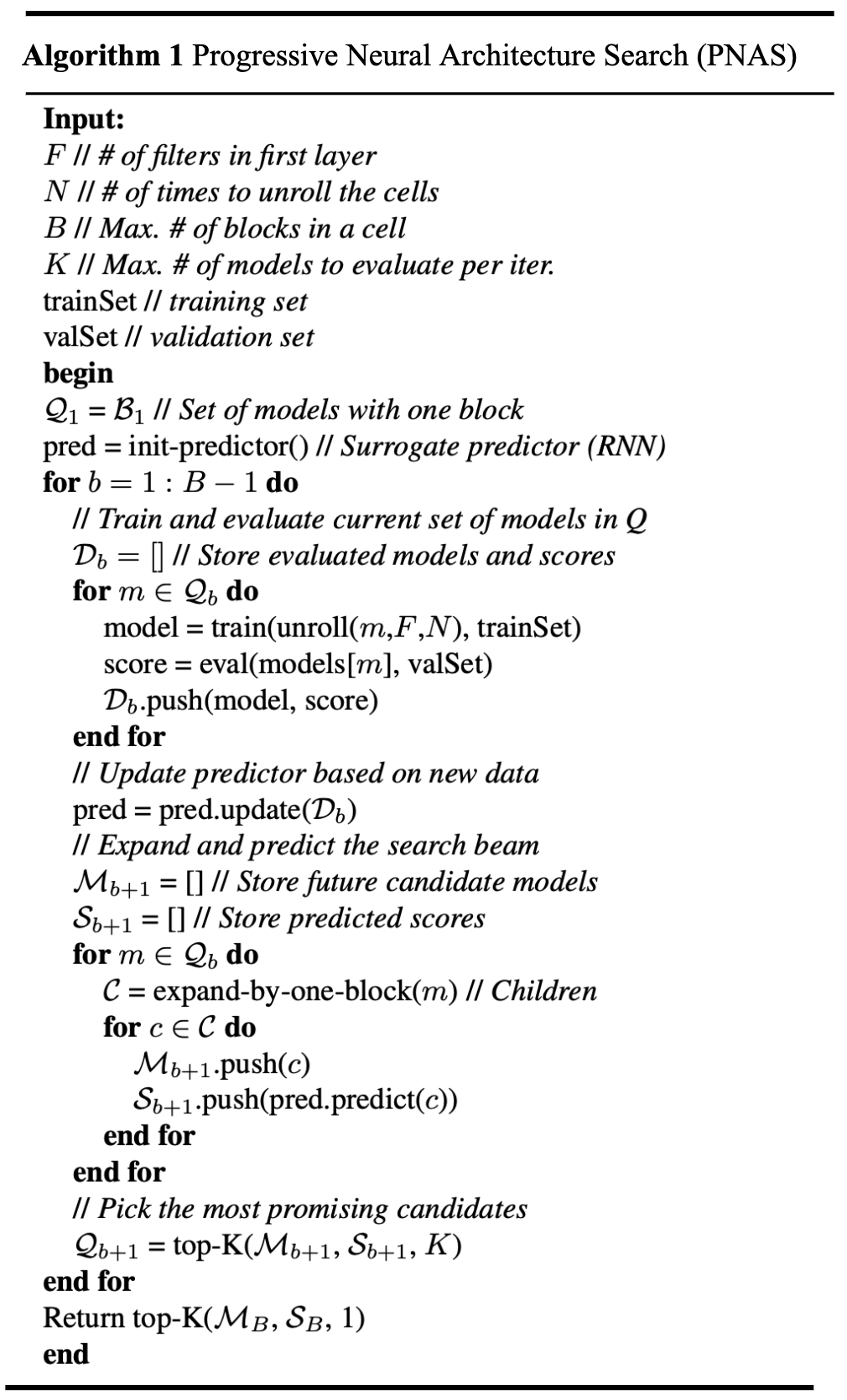
Progressive NAS (PNAS; Liu, et al 2018) frames NAS as a progressive procedure that searches architectures of increasing complexity. Rather than using RL or EA, PNAS adopts Sequential Model-based Bayesian Optimization (SMBO) as its search strategy. PNAS is similar to A* search because it explores models from simple to complex while learning a surrogate function that guides which candidates to evaluate next.
A* search algorithm (“best-first search”) is a popular algorithm for path finding. The problem is framed as finding a path of smallest cost from a specific starting node to a given target node in a weighted graph. At each iteration, A* finds a path to extend by minimizing: $f(n)=g(n)+h(n)$, where $n$ is the next node, $g(n)$ is the cost from start to $n$, and $h(n)$ is the heuristic function that estimates the minimum cost of going from node $n$ to the goal.
PNAS uses the NASNet search space. Each block is represented as a 5-element tuple, and PNAS restricts step 5 to use only element-wise addition as the combination operator (no concatenation). In contrast to fixing the number of blocks $B$, PNAS begins with $B=1$, namely a model whose cell contains only one block, and then increases $B$ progressively.
Validation-set performance is used as feedback to train a surrogate model that predicts the performance of new architectures. With this predictor, the method can decide which models should be prioritized for evaluation next. Because the performance predictor must support variable-sized inputs, provide accurate estimates, and be sample-efficient, they ultimately use an RNN.
Gradient descent
Applying gradient descent to update the architecture search model requires making the discrete operation-selection process differentiable. These methods typically combine learning the architecture parameters and the network weights within a single model. See more in the section on the “one-shot” approach.
Evaluation Strategy
To provide feedback for optimizing the search algorithm, we must measure, estimate, or predict each child model’s performance. Because candidate evaluation can be very expensive, many evaluation methods have been proposed to reduce time or computation. When evaluating a child model, the primary concern is typically accuracy on a validation set. Recent work has also begun to consider other properties, such as model size and latency, because some devices impose memory constraints or require fast response times.
Training from Scratch
The most straightforward approach is to train each child network independently from scratch until convergence and then measure validation accuracy (Zoph & Le 2017). Although this yields reliable performance numbers, each full train-to-converge-to-evaluate run produces only a single training sample for the RL controller (and RL is generally sample-inefficient). As a result, this approach is extremely expensive computationally.
Proxy Task Performance
Several methods use proxy task performance as a cheaper and faster estimator of a child network’s performance:
- Train on a smaller dataset.
- Train for fewer epochs.
- During the search stage, train and evaluate a down-scaled model. For example, after learning a cell structure, we can vary the number of cell repeats or scale up the number of filters (Zoph et al. 2018).
- Predict the learning curve. Baker et al (2018) formulate validation-accuracy prediction as a time-series regression problem. Features for the regression model ($\nu$-support vector machine regressions; $\nu$-SVR) include early sequences of per-epoch accuracy, architecture parameters, and hyperparameters.
Parameter Sharing
Rather than training each child model independently from scratch, a natural question is whether we can deliberately introduce dependencies among child models and reuse weights across them. Several researchers have demonstrated that this strategy can be effective.
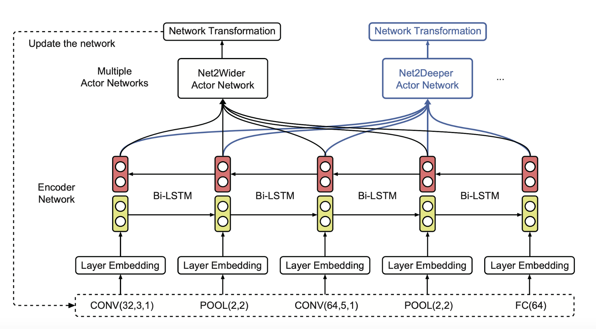
Building on the Net2net transformation, Cai et al (2017) proposed Efficient Architecture Search (EAS). EAS uses a reinforcement learning (RL) agent, referred to as a meta-controller, to predict function-preserving network transformations that expand network depth or increase layer width. Because the network is grown incrementally, weights from previously validated networks can be reused during subsequent exploration. With inherited weights, newly generated networks require only light-weight training.
The meta-controller learns to produce network transformation actions conditioned on the current architecture, which is represented as a variable-length string. To accommodate variable-length architecture descriptions, the meta-controller is implemented as a bidirectional recurrent network. Multiple actor networks produce different transformation decisions:
- Net2WiderNet replaces a layer with a wider layer (more units for fully connected layers, or more filters for convolutional layers) while preserving the original function.
- Net2DeeperNet inserts a new layer initialized to add an identity mapping between two layers, thereby preserving the function.
Motivated by a closely related idea, Efficient NAS (ENAS; Pham et al. 2018) accelerates NAS (i.e. 1000x less) by aggressively sharing parameters across child models. ENAS is driven by the observation that all sampled architecture graphs can be interpreted as sub-graphs of a larger supergraph. All child networks share the weights of this supergraph.

ENAS alternates between training the shared model weights $\omega$ and training the controller $\theta$:
- The controller LSTM parameters $\theta$ are trained with REINFORCE, where the reward $R(\mathbf{m}, \omega)$ is computed on the validation set.
- The shared child-model parameters $\omega$ are trained using a standard supervised learning loss. Note that different operators associated with the same node in the supergraph maintain distinct parameters.
Prediction-Based
In a typical child-model evaluation loop, model weights are updated via standard gradient descent. SMASH (Brock et al. 2017) introduces a different and intriguing question: Can we directly predict model weights from the network architecture parameters?
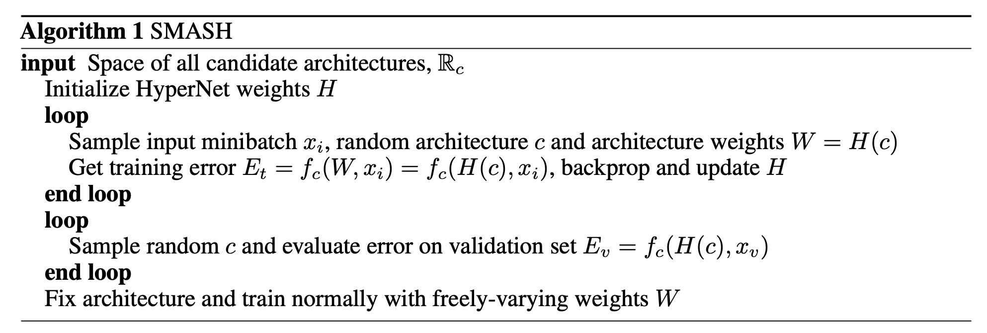
SMASH uses a HyperNet (Ha et al 2016) to generate a model’s weights directly, conditioned on an encoding of the model’s architecture configuration. The model is then validated using the HyperNet-generated weights. In this setup, no additional training is required for each child model, but the HyperNet itself must be trained.
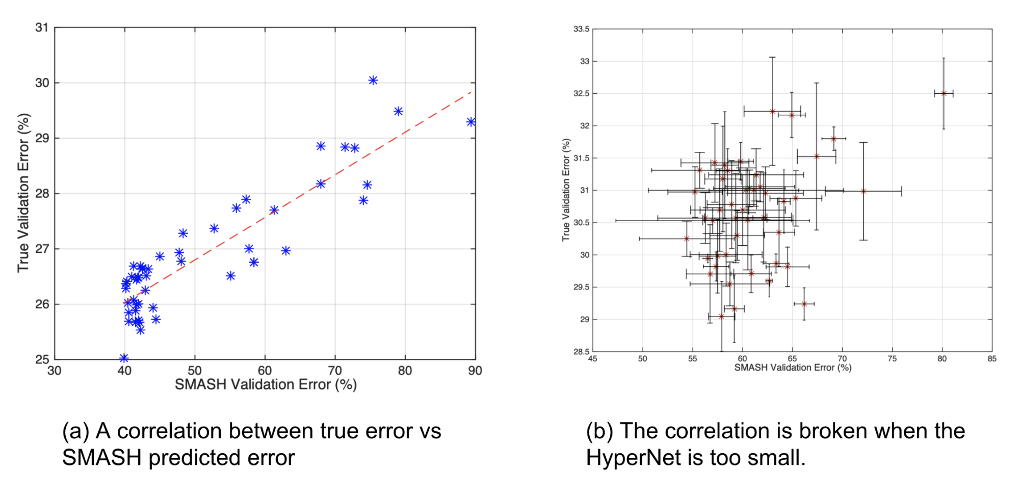
The relationship between performance obtained with SMASH-generated weights and true validation error indicates that predicted weights can, to some extent, support model comparison. However, the HyperNet must have sufficient capacity, because this correlation degrades if the HyperNet is too small relative to the child model.
SMASH can be interpreted as an alternative implementation of parameter sharing. One limitation of SMASH, noted by Pham et al. (2018), is that using a HyperNet restricts SMASH child-model weights to a low-rank space, because the weights are generated via tensor products. In contrast, ENAS does not impose this restriction.
One-Shot Approach: Search + Evaluation
Conducting search and evaluation independently over a large population of child models is expensive. Promising approaches such as Brock et al. (2017) and Pham et al. (2018) show that training a single model can be sufficient to emulate any child model in the search space.
One-shot architecture search extends weight sharing by coupling architecture generation learning with weight learning. The approaches below all treat child architectures as distinct sub-graphs of a supergraph, sharing weights across common edges in that supergraph.
Bender et al (2018) build a single, large, over-parameterized network, referred to as the One-Shot model, designed to include every candidate operation in the search space. Using ScheduledDropPath (the dropout rate increases over time, reaching $r^{1/k}$ at the end of training, where $0 < r < 1$ is a hyperparam and $k$ is the number of incoming paths) along with carefully selected techniques (e.g. ghost batch normalization, and L2 regularization applied only to the active architecture), training of this very large model can be sufficiently stabilized and then used to evaluate any child model sampled from the supergraph.
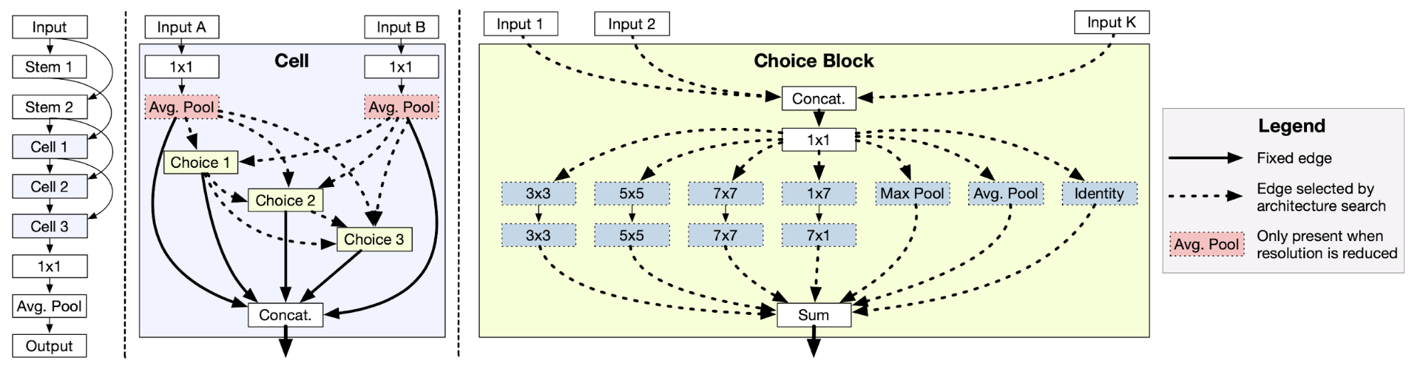
After training the one-shot model, it can evaluate many architectures sampled at random by zeroing out or removing selected operations. This random sampling procedure can be replaced with RL or evolutionary methods.
Bender et al. observed that accuracy measured using the one-shot model can differ substantially from the accuracy of the same architecture after modest fine-tuning. Their hypothesis is that the one-shot model implicitly learns to emphasize the most useful operations and to rely on them when available. As a result, zeroing out useful operations can sharply reduce accuracy, whereas removing less important components has only minor impact. Consequently, evaluation using the one-shot model exhibits higher variance in scores.
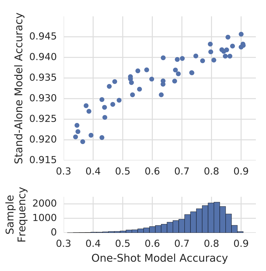
Although constructing such a search graph is clearly nontrivial, the results highlight the potential of the one-shot approach. Notably, it can perform well using gradient descent alone, without requiring an additional method such as RL or EA.
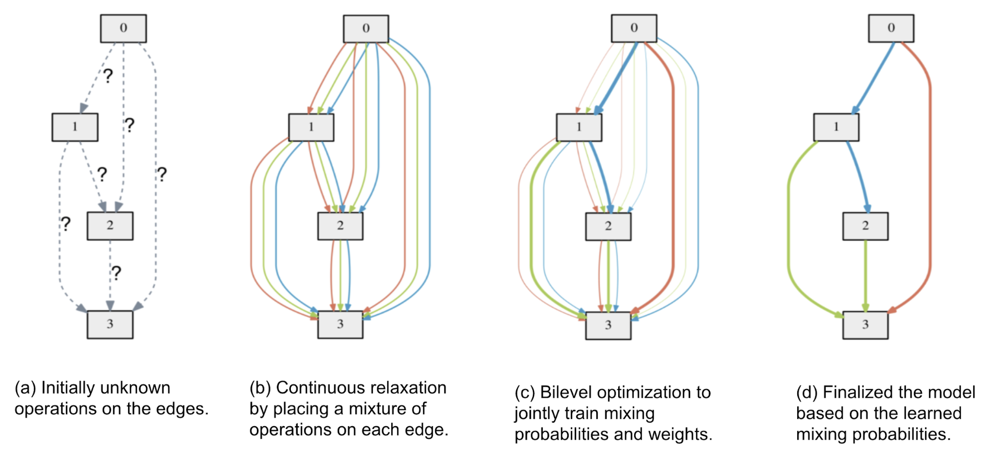
One widely held view is that a major source of NAS inefficiency is treating architecture search as black-box optimization, which leads to methods such as RL, evolution, SMBO, and others. If, instead, we rely on standard gradient descent, the search process may become more efficient. Along these lines, Liu et al (2019) introduced Differentiable Architecture Search (DARTS). DARTS applies a continuous relaxation to each path in the supergraph, enabling joint optimization of architecture parameters and weights via gradient descent.
Using the directed acyclic graph (DAG) formulation, a cell is represented as a DAG consisting of a topologically ordered sequence of $N$ nodes. Each node has a latent representation $x_i$ to be learned. Each edge $(i, j)$ is associated with an operation $o^{(i,j)} \in \mathcal{O}$ that transforms $x_j$ to form $x_i$:
To make the search space continuous, DARTS replaces the categorical selection of a specific operation with a softmax over all operations, reducing architecture search to learning a set of mixing probabilities $\alpha = \{ \alpha^{(i,j)} \}$.
where $\alpha_{ij}$ is a vector of dimension $\vert \mathcal{O} \vert$, containing weights between nodes $i$ and $j$ over different operations.
This yields a bilevel optimization problem, since we aim to optimize both the network weights $w$ and the architecture representation $\alpha$:
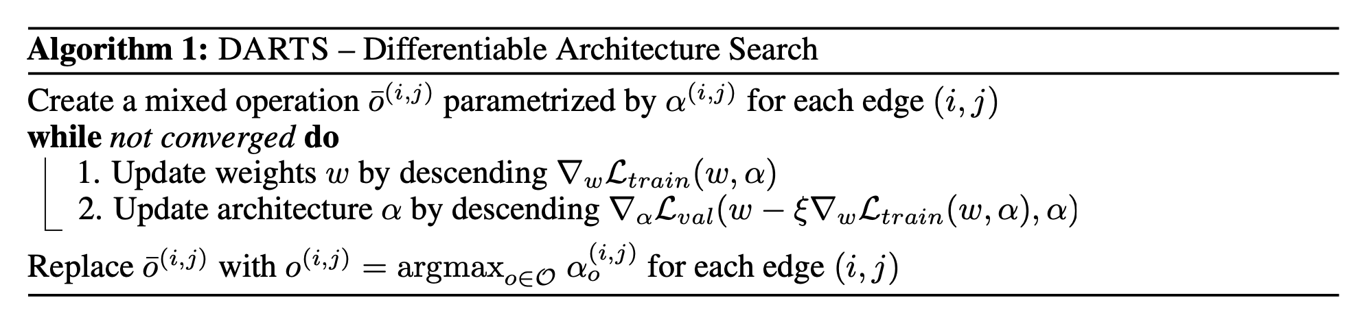
At step $k$, given the current architecture parameters $\alpha_{k−1}$, we first optimize the weights $w_k$ by updating $w_{k−1}$ in the direction that minimizes the training loss $\mathcal{L}_\text{train}(w_{k−1}, \alpha_{k−1})$ with learning rate $\xi$. Next, holding the newly updated weights $w_k$ fixed, we update the mixing probabilities to minimize the validation loss after a single step of gradient descent w.r.t. the weights:
The key motivation is to identify an architecture that achieves low validation loss when its weights are optimized by gradient descent, with the one-step unrolled weights acting as a surrogate for $w^∗(\alpha)$.
Side note: Earlier we have seen similar formulation in MAML where the two-step optimization happens between task losses and the meta-learner update, as well as framing Domain Randomization as a bilevel optimization for better transfer in the real environment.
where the red part is using numerical differentiation approximation where $w_k^+ = w_k + \epsilon \nabla_{w’_k} \mathcal{L}_\text{val}(w’_k, \alpha_{k-1})$ and $w_k^- = w_k - \epsilon \nabla_{w’_k} \mathcal{L}_\text{val}(w’_k, \alpha_{k-1})$.
In a related direction, Stochastic NAS (Xie et al., 2019) introduces a continuous relaxation using the concrete distribution (CONCRETE = CONtinuous relaxations of disCRETE random variables; Maddison et al 2017) together with reparametrization tricks. The objective matches DARTS: make the discrete distribution differentiable to enable optimization via gradient descent.
- TBA: maybe add more details on SNASDARTS can substantially reduce GPU-hour costs. In their CNN-cell search experiments, they report $N=7$ and require only 1.5 days on a single GPU. However, DARTS also incurs high GPU memory usage due to its continuous architecture representation. To fit the model within the memory constraints of a single GPU, they selected a small $N$.
To limit GPU memory usage, ProxylessNAS (Cai et al., 2019) frames NAS as a path-level pruning process in a DAG and binarizes architecture parameters so that only one path between two nodes is active at any time. The probability that an edge is masked or unmasked is learned by sampling a small number of binarized architectures and updating the corresponding probabilities using BinaryConnect (Courbariaux et al., 2015). ProxylessNAS highlights a strong connection between NAS and model compression. Through path-level compression, it reduces memory consumption by an order of magnitude.
Continuing with the graph representation, consider a DAG adjacency matrix $G$, where $G_{ij}$ denotes an edge between node $i$ and node $j$, and the edge value is selected from a set of $\vert \mathcal{O} \vert$ candidate primitive operations, $\mathcal{O} = \{ o_1, \dots \}$. The One-Shot model, DARTS, and ProxylessNAS all represent each edge as a mixture of operations, $m_\mathcal{O}$, but differ in their specific formulations.
In the One-Shot model, $m_\mathcal{O}(x)$ is the sum of all operations. In DARTS, it is a weighted sum, where weights are computed by applying softmax to a real-valued architecture-weighting vector $\alpha$ of length $\vert \mathcal{O} \vert$. ProxylessNAS converts the softmax probabilities $\alpha$ into a binary gate, using that gate to keep only one operation active at a time.
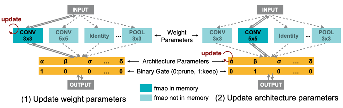
ProxylessNAS alternates between two training steps:
- When training weight parameters $w$, it freezes architecture parameters $\alpha$ and stochastically samples binary gates $g$ according to $m^\text{binary}_\mathcal{O}(x)$ above. The weight parameters are then updated using standard gradient descent.
- When training architecture parameters $\alpha$, it freezes $w$, resets the binary gates, and then updates $\alpha$ on the validation set. Following the BinaryConnect approach, the gradient w.r.t. architecture parameters can be approximated by using $\partial \mathcal{L} / \partial g_i$ in place of $\partial \mathcal{L} / \partial p_i$:
Instead of BinaryConnect, REINFORCE can also be used to update parameters by maximizing reward, and no RNN meta-controller is required.
Computing $\partial \mathcal{L} / \partial g_i$ requires calculating and storing $o_i(x)$, which consumes $\vert \mathcal{O} \vert$ times GPU memory. To address this, ProxylessNAS factorizes the selection of one path out of $N$ into multiple binary selection tasks (intuition: “if a path is the best choice, it should be better than any other path”). At each update step, only two paths are sampled while all others are masked. The two selected paths are updated according to the equation above, then scaled appropriately so that the weights of the other paths remain unchanged. After this procedure, one of the sampled paths is strengthened (its path weight increases) and the other is weakened (its path weight decreases), while all remaining paths are left unchanged.
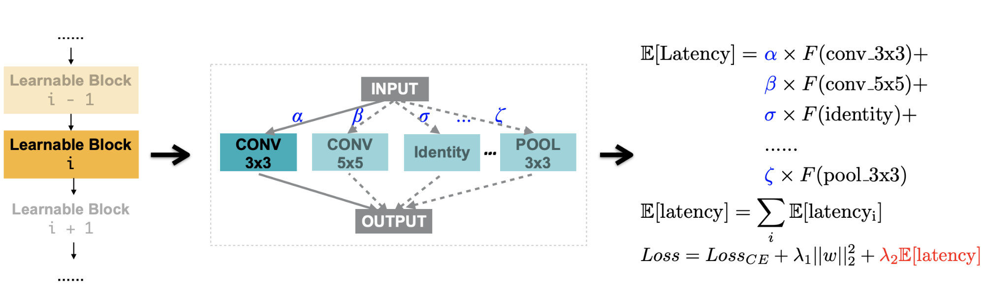
In addition to accuracy, ProxylessNAS treats latency as an important optimization objective, since different devices can impose very different inference latency constraints (e.g. GPU, CPU, mobile). To make latency differentiable, latency is modeled as a continuous function of network dimensions. The expected latency of a mixed operation can be expressed as $\mathbb{E}[\text{latency}] = \sum_j p_j F(o_j)$, where $F(.)$ is a latency prediction model:
What’s the Future?
To this point, we have reviewed many compelling ideas for automating network architecture engineering through neural architecture search, and many of these methods have achieved impressive performance. However, it remains challenging to infer why certain architectures perform well and how to develop modules that generalize across tasks, rather than being tightly tailored to a particular dataset.
As also noted in Elsken, et al (2019):
“…, so far it provides little insights into why specific architectures work well and how similar the architectures derived in independent runs would be. Identifying common motifs, providing an understanding why those motifs are important for high performance, and investigating if these motifs generalize over different problems would be desirable.”
At the same time, focusing exclusively on validation accuracy may be insufficient (Cai et al., 2019). Devices such as mobile phones, which are used daily, typically have limited memory and compute capacity. As AI applications increasingly influence daily life, a more device-specific perspective becomes unavoidable.
Another interesting line of inquiry is to incorporate unlabelled dataset and self-supervised learning into NAS. Labeled datasets are always limited, and it can be difficult to assess whether a labeled dataset contains biases or deviates substantially from real-world data distributions.
Liu et al (2020) investigate the question “Can we find high-quality neural architecture without human-annotated labels?” and propose a setup called Unsupervised Neural Architecture Search (UnNAS). In this framework, architecture quality must be estimated in an unsupervised manner during the search phase. The paper evaluates three unsupervised pretext tasks: image rotation prediction, colorization, and solving the jigsaw puzzle.
Across a set of UnNAS experiments, they report the following observations:
- High rank correlation between supervised accuracy and pretext accuracy on the same dataset. Typically the rank correlation exceeds 0.8, regardless of dataset, search space, or pretext task.
- High rank correlation between supervised accuracy and pretext accuracy across datasets.
- Higher pretext accuracy translates into higher supervised accuracy.
- UnNAS architectures achieve performance comparable to supervised counterparts, although not better yet.
One hypothesis is that architecture quality correlates with image statistics. Since CIFAR-10 and ImageNet both consist of natural images, they are comparable, making results transferable. UnNAS could enable using a much larger volume of unlabeled data during the search phase, potentially capturing image statistics more effectively.
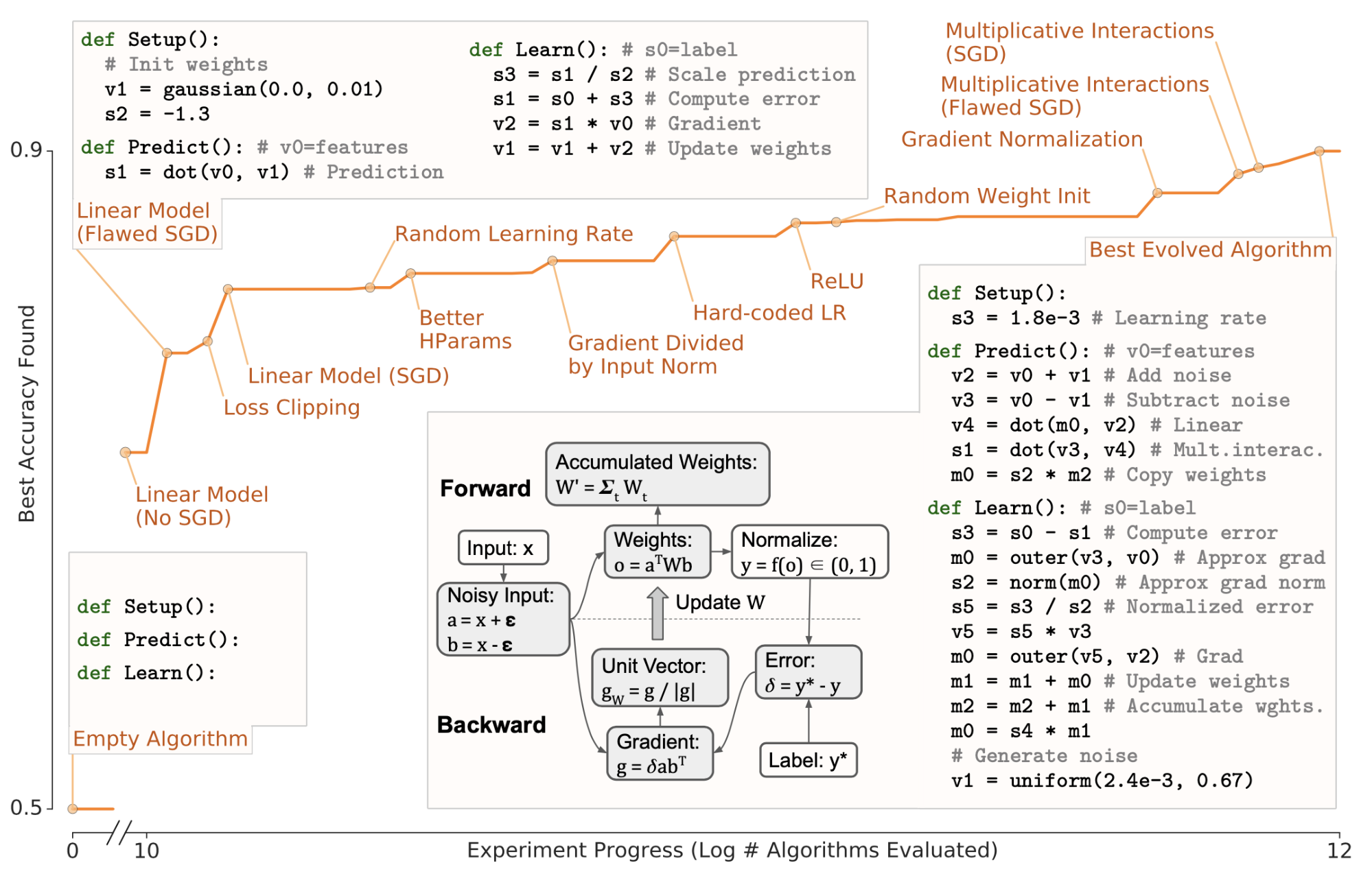
Hyperparameter search has long been a central topic in the ML community, and NAS automates architecture engineering. Over time, we have increasingly automated ML processes that typically require substantial human effort. Extending this trajectory further raises an additional question: can ML algorithms themselves be discovered automatically? AutoML-Zero (Real et al 2020) explores this idea. Using aging evolutionary algorithms, AutoML-Zero searches over entire ML algorithms with minimal restrictions on form, relying only on simple mathematical operations as building blocks.
AutoML-Zero learns three component functions, each defined using only very basic operations.
Setup: initialize memory variables (weights).Learn: modify memory variablesPredict: produce a prediction from an input $x$.
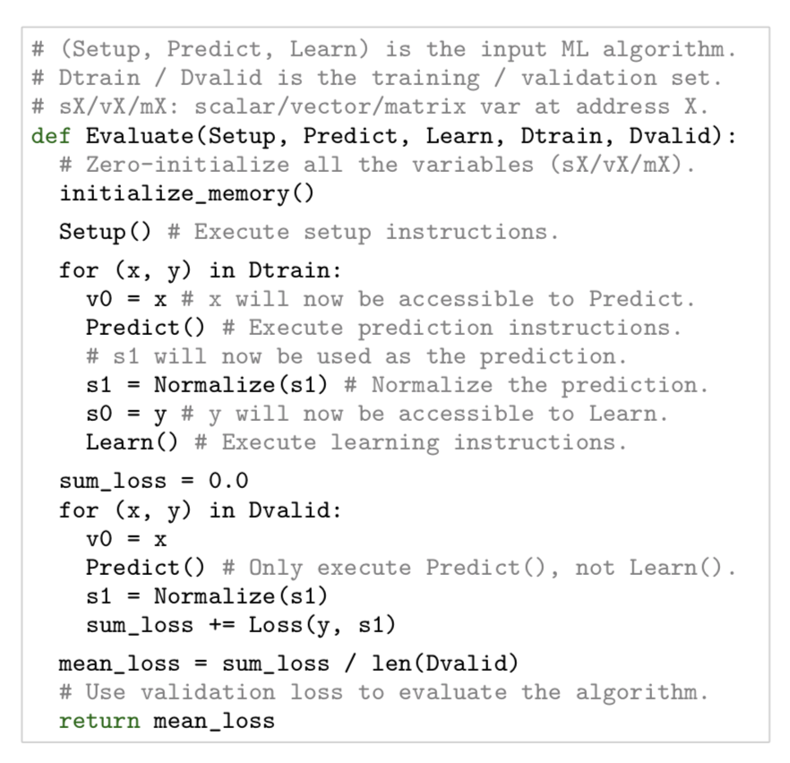
When mutating a parent genotype, three categories of operations are used:
- Insert a random instruction or remove an instruction at a random location in a component function;
- Randomize all the instructions in a component function;
- Modify one of the arguments of an instruction by replacing it with a random choice (e.g. “swap the output address” or “change the value of a constant”)
Appendix: Summary of NAS Papers
| Model name | Search space | Search algorithms | Child model evaluation |
|---|---|---|---|
| NEAT (2002) | - | Evolution (Genetic algorithm) | - |
| NAS (2017) | Sequential layer-wise ops | RL (REINFORCE) | Train from scratch until convergence |
| MetaQNN (2017) | Sequential layer-wise ops | RL (Q-learning with $\epsilon$-greedy) | Train for 20 epochs |
| HNAS (2017) | Hierarchical structure | Evolution (Tournament selection) | Train for a fixed number of iterations |
| NASNet (2018) | Cell-based | RL (PPO) | Train for 20 epochs |
| AmoebaNet (2018) | NASNet search space | Evolution (Tournament selection with aging regularization) | Train for 25 epochs |
| EAS (2018a) | Network transformation | RL (REINFORCE) | 2-stage training |
| PNAS (2018) | Reduced version of NASNet search space | SMBO; Progressive search for architectures of increasing complexity | Train for 20 epochs |
| ENAS (2018) | Both sequential and cell-based search space | RL (REINFORCE) | Train one model with shared weights |
| SMASH (2017) | Memory-bank representation | Random search | HyperNet predicts weights of evaluated architectures. |
| One-Shot (2018) | An over-parameterized one-shot model | Random search (zero out some paths at random) | Train the one-shot model |
| DARTS (2019) | NASNet search space | Gradient descent (Softmax weights over operations) | |
| ProxylessNAS (2019) | Tree structure architecture | Gradient descent (BinaryConnect) or REINFORCE | |
| SNAS (2019) | NASNet search space | Gradient descent (concrete distribution) | |
Citation
Please cite this post as follows:
Weng, Lilian. (Aug 2020). Neural architecture search. Lil’Log. https://lilianweng.github.io/posts/2020-08-06-nas/.
Alternatively:
@article{weng2020nas,
  title   = "Neural Architecture Search",
  author  = "Weng, Lilian",
  journal = "lilianweng.github.io",
  year    = "2020",
  month   = "Aug",
  url     = "https://lilianweng.github.io/posts/2020-08-06-nas/"
}
Reference
[1] Thomas Elsken, Jan Hendrik Metzen, Frank Hutter. “Neural Architecture Search: A Survey” JMLR 20 (2019) 1-21.
[2] Kenneth O. Stanley, et al. “Designing neural networks through neuroevolution” Nature Machine Intelligence volume 1, pages 24–35 (2019).
[3] Kenneth O. Stanley & Risto Miikkulainen. “Evolving Neural Networks through Augmenting Topologies” Evolutionary Computation 10(2): 99-127 (2002).
[4] Barret Zoph, Quoc V. Le. “Neural architecture search with reinforcement learning” ICLR 2017.
[5] Bowen Baker, et al. “Designing Neural Network Architectures using Reinforcement Learning” ICLR 2017.
[6] Bowen Baker, et al. “Accelerating neural architecture search using performance prediction” ICLR Workshop 2018.
[7] Barret Zoph, et al. “Learning transferable architectures for scalable image recognition” CVPR 2018.
[8] Hanxiao Liu, et al. “Hierarchical representations for efficient architecture search.” ICLR 2018.
[9] Esteban Real, et al. “Regularized Evolution for Image Classifier Architecture Search” arXiv:1802.01548 (2018).
[10] Han Cai, et al. [“Efficient architecture search by network transformation”] AAAI 2018a.
[11] Han Cai, et al. “Path-Level Network Transformation for Efficient Architecture Search” ICML 2018b.
[12] Han Cai, Ligeng Zhu & Song Han. “ProxylessNAS: Direct Neural Architecture Search on Target Task and Hardware” ICLR 2019.
[13] Chenxi Liu, et al. “Progressive neural architecture search” ECCV 2018.
[14] Hieu Pham, et al. “Efficient neural architecture search via parameter sharing” ICML 2018.
[15] Andrew Brock, et al. “SMASH: One-shot model architecture search through hypernetworks.” ICLR 2018.
[16] Gabriel Bender, et al. “Understanding and simplifying one-shot architecture search.” ICML 2018.
[17] Hanxiao Liu, Karen Simonyan, Yiming Yang. “DARTS: Differentiable Architecture Search” ICLR 2019.
[18] Sirui Xie, Hehui Zheng, Chunxiao Liu, Liang Lin. “SNAS: Stochastic Neural Architecture Search” ICLR 2019.
[19] Chenxi Liu et al. “Are Labels Necessary for Neural Architecture Search?” ECCV 2020.
[20] Esteban Real, et al. “AutoML-Zero: Evolving Machine Learning Algorithms From Scratch” ICML 2020.