[Updated on 2021-02-01: Updated to version 2.0 with several works added and many typos fixed.]
[Updated on 2021-05-26: Added P-tuning and Prompt Tuning in the “prompt design” section.]
[Updated on 2021-09-19: Added “unlikelihood training”.]

There is a gigantic amount of free text on the Web, several orders of magnitude more than labeled benchmark datasets. State-of-the-art language models (LMs) are trained on large-scale unsupervised Web data. When generating samples from an LM by iteratively sampling the next token, we have limited control over attributes of the output text, such as the topic, style, sentiment, etc. Many applications require strong control over model outputs. For example, if we plan to use an LM to generate reading materials for kids, we would like to guide the output stories to be safe, educational, and easily understood by children.

How can we steer a powerful unconditioned language model? In this post, we will delve into several approaches for controlled content generation with an unconditioned language model. Note that model steerability remains an open research question. Each method introduced has certain pros and cons.

1. Apply guided decoding strategies and select desired outputs at test time.
2. Optimize for the most desired outcomes through effective prompt design.
3. Fine-tune the base model or steerable layers to enable conditioned content generation.

In the following discussion, we assume we have access to a pretrained generative language model $p_\theta$. The model has learned the distribution over token sequences by optimizing next-token prediction: $ \mathcal{L}_\text{ML} = - \sum_t \log p_\theta(x_t \vert x_{<t}) $.

Decoding Strategies

By adopting different decoding methods, we can impose restrictions or preferences on the sampling process to alter generated samples without modifying any model weights. Although decoding strategies do not change the values of any trainable parameters, they are a quite important component.

Common Decoding Methods

Since the model’s final layer predicts logits $o$ over the vocabulary space, the next token can be sampled by applying softmax with temperature $T$. The probability of sampling the $i$-th token is

A low temperature makes the distribution sharper, while a high temperature makes it softer.

Greedy search: Always pick the next token with the highest probability, equivalent to setting temperature $T=0$. However, it tends to produce repeated phrases, even for well-trained models.

Beam search: It essentially performs breadth-first search, one token per tree level, but with limited bandwidth. At each level of the search tree, beam search keeps track of $n$ (called the “beam width”) best candidates and expands all successors of these candidates at the next level. Beam search can stop expanding a node if it reaches the EOS (end-of-sentence) token.

However, maximization-based decoding does not guarantee high-quality generation.

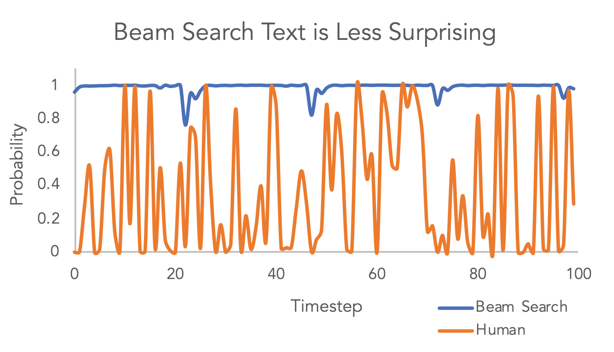
Top-k sampling (Fan et al., 2018): At each sampling step, only the top $k$ most likely tokens are selected, and the probability mass is redistributed among them. In Fan et al., 2018, the authors proposed using top-k random sampling in which the next token is randomly selected from among the top $k$ most likely candidates, and they argued that this approach can generate more novel and less repetitive content than beam search.

Nucleus sampling (Holtzman et al. 2019): Also known as “Top-p sampling”. One drawback of top-k sampling is that the predefined number $k$ does not take into consideration how skewed the probability distribution may be. Nucleus sampling selects the smallest set of top candidates whose cumulative probability exceeds a threshold (e.g., 0.95), and then rescales the distribution among the selected candidates.

With a proper set of hyperparameters, both top-k and nucleus sampling exhibit fewer repetitions.

Penalized sampling (Keskar et al. 2019): To avoid the common failure case of generating duplicate substrings, the CTRL paper proposed a new sampling method that penalizes repetition by discounting the scores of previously generated tokens. The probability distribution for the next token with a repetition penalty is defined as:

where $g$ contains a set of previously generated tokens, and $\mathbb{1}(.)$ is an identity function. $\theta=1.2$ was found to yield a good balance between reduced repetition and truthful generation.

Guided Decoding

All the standard decoding strategies above sample tokens according to the predicted probabilities, without additional information. Our preferences regarding topic or sentiment can be incorporated into the candidate ranking function to guide sample generation by altering the candidate ranking score. The ranking score for token selection at each decoding step can be defined as a combination of LM log-likelihood and a set of desired feature discriminators. The features are designed to quantify human preferences via heuristics (Ghazvininejad et al., 2017), supervised learning (Holtzman et al., 2018) or RL (Li et al., 2017).

Ghazvininejad et al. (2017) built a system called “Hafez” to generate poetry in a desired style by adjusting sampling weights in beam search during decoding. The likelihood of sampling the next token $x_{t+1}$ at step $t$ is augmented by a scoring function:

where $\log p(x_{t+1})$ is the log-likelihood predicted by the LM. $\text{score}(b_t)$ is the accumulated score of the words already generated in the current beam state $b_t$. The green part can incorporate many different features for steering the style of the output. A set of feature functions $f_i(.)$ define the preferences, and the associated weights $alpha_i$ act like “control knobs” that can be easily customized at decoding time. Features can measure a variety of attributes and can be easily combined; for example,

• whether $x_{t+1}$ exists in a bag of desired or banned topical words.
• whether $x_{t+1}$ indicates certain sentiments.
• whether $x_{t+1}$ is a repeated token (so $f_i$ needs to take the history as input as well).
• the length of $x_{t+1}$, if longer or shorter words are particularly preferred.

Similar to Hafez, Baheti et al. (2018) manually designed features for ranking and altered the sampling distribution by appending similarity scores between the topic distributions or embeddings of the context and the completion.

Holtzman et al. (2018) adopted a set of learned discriminators, each specializing in a different principle of communication guided by Grice’s maxims: quality, quantity, relation, and manner. The discriminators learn to encode these desired principles by measuring repetition, entailment, relevance, and lexical diversity, respectively. Given some ground-truth completion, all discriminator models are trained to minimize the ranking log-likelihood, $\log\sigma(f_i(y_g) - f_i(y))$, because the gold continuation $y_g$ is expected to receive a higher score than the generated continuation $y$. The weight coefficients $\alpha_i$ are also learned to minimize the score difference between the gold standard and the generated completion. Discriminative Adversarial Search (DAS; Scialom et al., 2020) is inspired by GANs and trains the discriminator to distinguish human-created text from machine-generated text. The discriminator predicts a label for each token rather than for the entire sequence. The discriminator log-probability is added to the score to guide sampling toward a human-written style.

Meister et al. (2020) studied beam search within a regularized decoding framework:

Since we expect maximum probability to correspond to minimum surprise, the surprisal of an LM at time step $t$ can be defined as follows:

The MAP (maximum a posteriori) term seeks sequences with maximum probability given the context, while the regularizer introduces other constraints. It is possible that a globally optimal strategy occasionally requires a high-surprisal step so that it can shorten the output length or produce more low-surprisal steps afterward.

Beam search has stood the test of time in NLP. The question is: If we want to model beam search as exact search in a regularized decoding framework, how should $\mathcal{R}(\mathbf{y})$ be modeled? The paper proposed a connection between beam search and the uniform information density (UID) hypothesis.

“The uniform information density hypothesis (UID; Levy and Jaeger, 2007) states that, subject to the constraints of grammar, humans prefer sentences that distribute information (in the information-theoretic sense) evenly across the linguistic signal, e.g., a sentence.”

In other words, it hypothesizes that humans prefer text with evenly distributed surprisal. Popular decoding methods like top-k sampling or nucleus sampling effectively filter out high-surprisal options, thus implicitly encouraging the UID property in output sequences.

The paper experimented with several forms of regularizers:

1. Greedy: $\mathcal{R}_\text{greedy}(\mathbf{y}) = \sum_{t=1}^{\vert\mathbf{y}\vert} \big(u_t(y_t) - \min_{y’ \in \mathcal{V}} u_t(y’) \big)^2$; if we set $\lambda \to \infty$, we obtain greedy search. Note that being greedy at each individual step does not guarantee global optimality.
2. Variance regularizer: $\mathcal{R}_\text{var}(\mathbf{y}) = \frac{1}{\vert\mathbf{y}\vert}\sum_{t=1}^{\vert\mathbf{y}\vert} \big(u_t(y_t) - \bar{u} \big)^2$ , where $\bar{u}$ is the average surprisal over all time steps. It directly encodes the UID hypothesis.
3. Local consistency: $\mathcal{R}_\text{local}(\mathbf{y}) = \frac{1}{\vert\mathbf{y}\vert}\sum_{t=1}^{\vert\mathbf{y}\vert} \big(u_t(y_t) - u_{t-1}(y_{t-1}) \big)^2$; this decoding regularizer encourages adjacent tokens to have similar surprisal.
4. Max regularizer: $\mathcal{R}_\text{max}(\mathbf{y}) = \max_t u_t(y_t)$ penalizes the maximum magnitude of surprisal.
5. Squared regularizer: $\mathcal{R}_\text{square}(\mathbf{y}) = \sum_{t=1}^{\vert\mathbf{y}\vert} u_t(y_t)^2$ encourages all tokens to have surprisal close to 0.

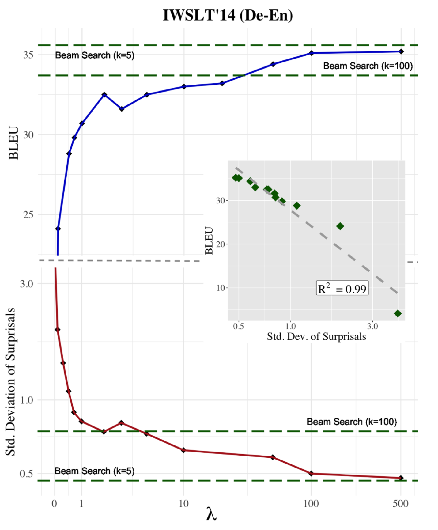
An experiment with greedy regularizers showed that larger $\lambda$ leads to better performance (e.g., measured by BLEU for the NMT task) and lower standard deviation of surprisal.

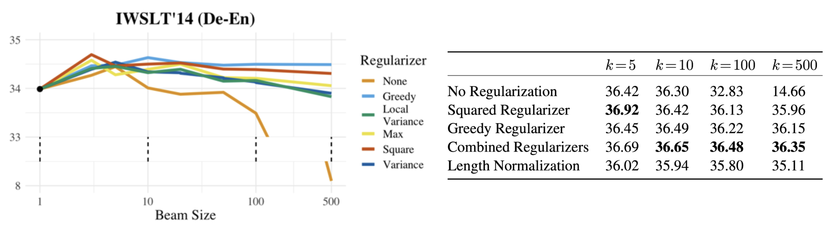
Default beam search tends to produce lower-quality text generation as beam size increases. Regularized beam search greatly helps alleviate this issue. A combined regularizer further improves performance. In their NMT experiments, they found that $\lambda=5$ for greedy and $\lambda=2$ for squared form the optimal combined regularizer.

Guided decoding essentially runs a more expensive beam search in which the sampling probability distribution is modified using side information about human preferences.

Trainable Decoding

Given a trained language model, Gu et al (2017) proposed a trainable greedy decoding algorithm to maximize an arbitrary objective for sampled sequences. The idea is based on noisy, parallel approximate decoding (NPAD). NPAD injects unstructured noise into the model’s hidden states and runs noisy decoding multiple times in parallel to avoid potential degradation. Going a step further, trainable greedy decoding replaces the unstructured noise with a learnable random variable predicted by an RL agent that takes the previous hidden state, the previously decoded token, and the context as input. In other words, the decoding algorithm learns an RL actor to manipulate the model’s hidden states for better outcomes.

Grover et al. (2019) trained a binary classifier to distinguish samples from the data distribution and samples from the generative model. This classifier is used to estimate importance weights for constructing a new unnormalized distribution. The proposed strategy is called likelihood-free importance weighting (LFIW).

Let $p$ be the real data distribution and $p_\theta$ a learned generative model. A classical approach for evaluating the expectation of a function $f$ under $p$ using samples from $p_\theta$ is importance sampling.

However, $p(\mathbf{x})$ can only be estimated from finite datasets. Let $c_\phi: \mathcal{X} \to [0,1]$ be a probabilistic binary classifier that predicts whether a sample $\mathbf{x}$ comes from the true data distribution ($y=1$). The joint distribution over $\mathcal{X}\times\mathcal{Y}$ is denoted as $q(\mathbf{x}, y)$.

Then, if $c_\phi$ is Bayes optimal, the importance weight can be estimated as:

where $\gamma = \frac{q(y=0)}{q(y=1)} > 0$ is a fixed odds ratio.

Because we cannot learn a perfectly optimal classifier, the importance weight is an estimate $\hat{w}_\phi$. A few practical tricks can be applied to mitigate cases where the classifier exploits artifacts in generated samples to make overly confident predictions (i.e., very small importance weights):

1. Self-normalization: normalize the weight by the sum, $\hat{w}_\phi(\mathbf{x}_i) / \sum_{j=1}^N \hat{w}_\phi(\mathbf{x}_j)$.
2. Flattening: add a power-scaling parameter $\alpha > 0$, $\hat{w}_\phi(\mathbf{x}_i)^\alpha$.
3. Clipping: specify a lower bound, $\max(\hat{w}_\phi(\mathbf{x}_i), \beta)$.

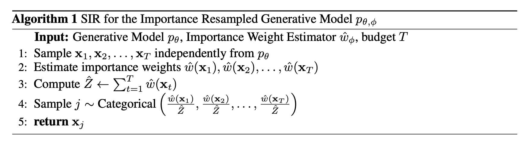
To sample from an importance-resampled generative model, $\mathbf{x}\sim p_{\theta, \phi}(\mathbf{x}) \propto p_\theta(\mathbf{x})\hat{w}_\phi(\mathbf{x})$, they adopt SIR (Sampling-Importance-Resampling),

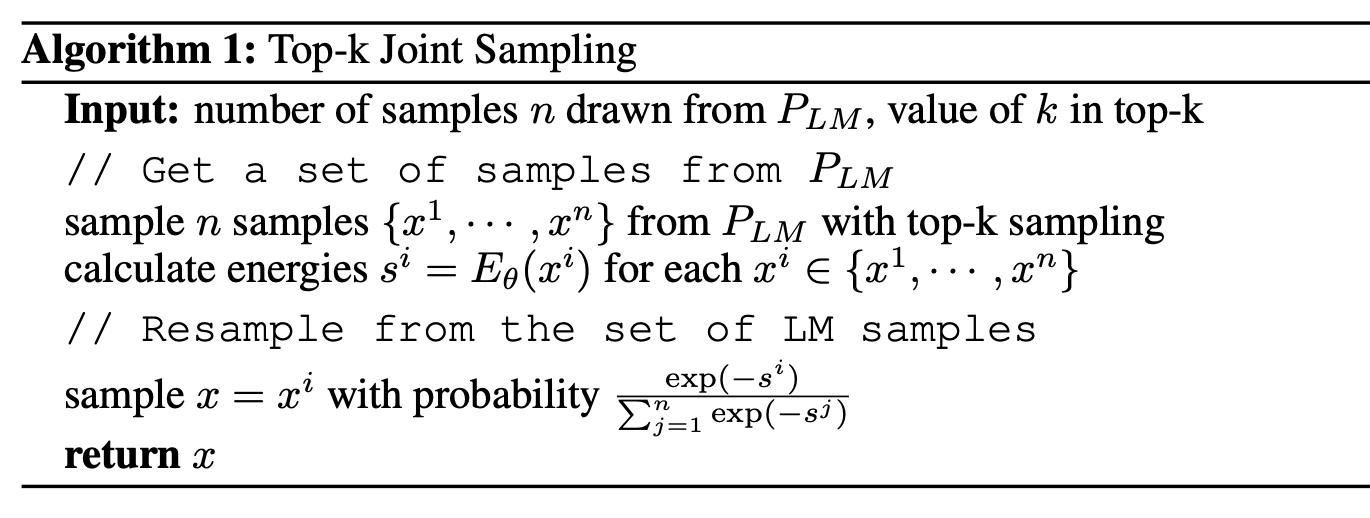
Deng et al., 2020 proposed learning an EBM to steer an LM in the residual space, $P_\theta(x) \propto P_\text{LM}(x)\exp(-E_\theta(x))$, where $P_\theta$ is the joint model and $E_\theta$ is the residual energy function to be learned. If we know the partition function $Z$, we can model the generative model for generating a sequence $x_{p+1}, \dots, x_T$ as:

The goal is to learn the parameters of the energy function $E_\theta$ so that the joint model $P_\theta$ becomes closer to the desired data distribution. The residual energy function is trained via noise-contrastive estimation (NCE), treating $P_\theta$ as the model distribution and $P_\text{LM}$ as the noise distribution:

However, the partition function is intractable in practice. The paper proposed a simple approach: first sample from the original LM and then resample those samples according to the energy function. Unfortunately, this is quite expensive.

Smart Prompt Design

Large language models have been shown to be very powerful on many NLP tasks, even with only prompting and no task-specific fine-tuning (GPT2, GPT3. Prompt design has a major impact on downstream-task performance and often requires time-consuming manual crafting. For example, factual questions can see a large boost with smart prompt design in a “closed-book exam” setting (Shin et al., 2020, Jiang et al., 2020)). I expect to see a growing body of literature on automatic smart prompt design.

Gradient-based Search

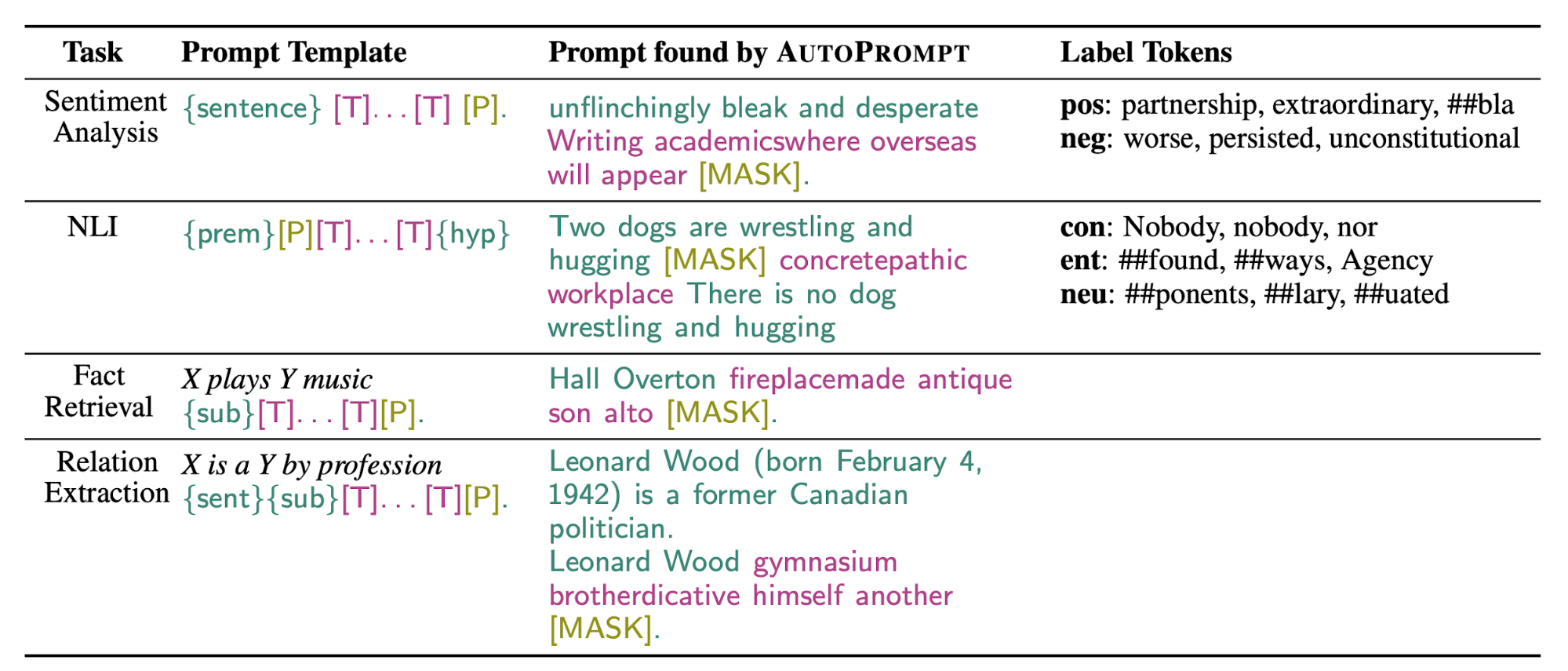
AutoPrompt (Shin et al., 2020; code) is a method for automatically creating prompts for various tasks via gradient-based search. AutoPrompt constructs a prompt by combining the original task inputs $x$ with a set of trigger tokens $x_\text{trig}$ according to a template $\lambda$. The trigger tokens are shared across all inputs and are therefore universally effective.

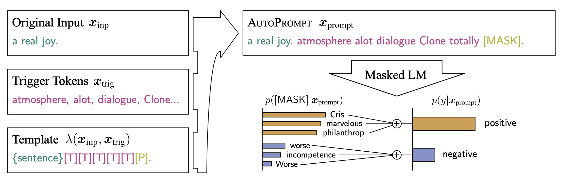
The universal trigger tokens are identified using a gradient-guided search strategy, as in Wallace et al., 2019. The universal setting means that the trigger tokens $x_\text{trig}$ can optimize the target output $\tilde{y}$ for all inputs from a dataset:

The search operates in embedding space. The embedding of each trigger token $e_{\text{trig}_i}$ is first initialized to a default value and then updated to minimize the first-order Taylor expansion of the task-specific loss around the current token embedding:

where $\mathcal{V}$ refers to the embedding matrix of all tokens. $\nabla_{e^{(t)}_{\text{trig}_i}} \mathcal{L}$ is the average gradient of the task loss over a batch at iteration $t$. We can brute-force the optimal $e$ via a $\vert \mathcal{V} \vert d$-dimensional dot product, which is inexpensive and can be computed in parallel.

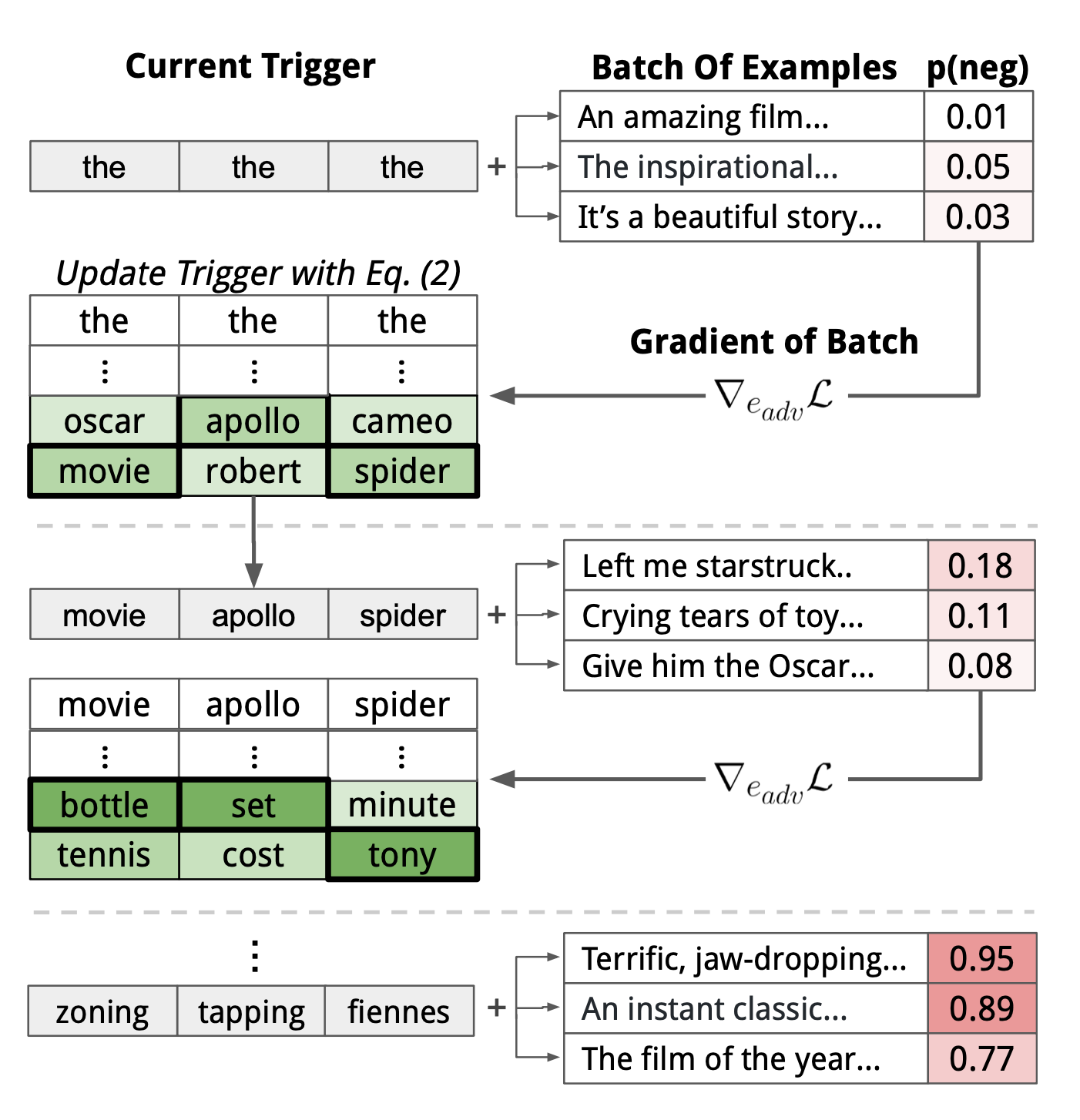
The token-replacement method above can be augmented with beam search. When searching for the optimal token embedding $e$, we can select top-$k$ candidates rather than a single one, search from left to right, and score each beam by $\mathcal{L}$ on the current data batch.

Smart prompt design essentially produces an efficient context that can lead to the desired completion. Motivated by this observation, Li & Liang (2021) proposed Prefix-Tuning which allocates a small number of trainable parameters at the beginning of an input sequence (called a “prefix”) to steer an LM, $[\text{PREFIX}; x; y]$. Let $\mathcal{P}_\text{idx}$ be a set of prefix indices and let $\text{dim}(h_i)$ be the embedding size. The prefix parameters $P_\theta$ have dimension $\vert\mathcal{P}_\text{idx}\vert \times \text{dim}(h_i)$, and the hidden state takes the form:

Note that only $P_\theta$ is trainable, and the LM parameters $\phi$ are frozen during training.

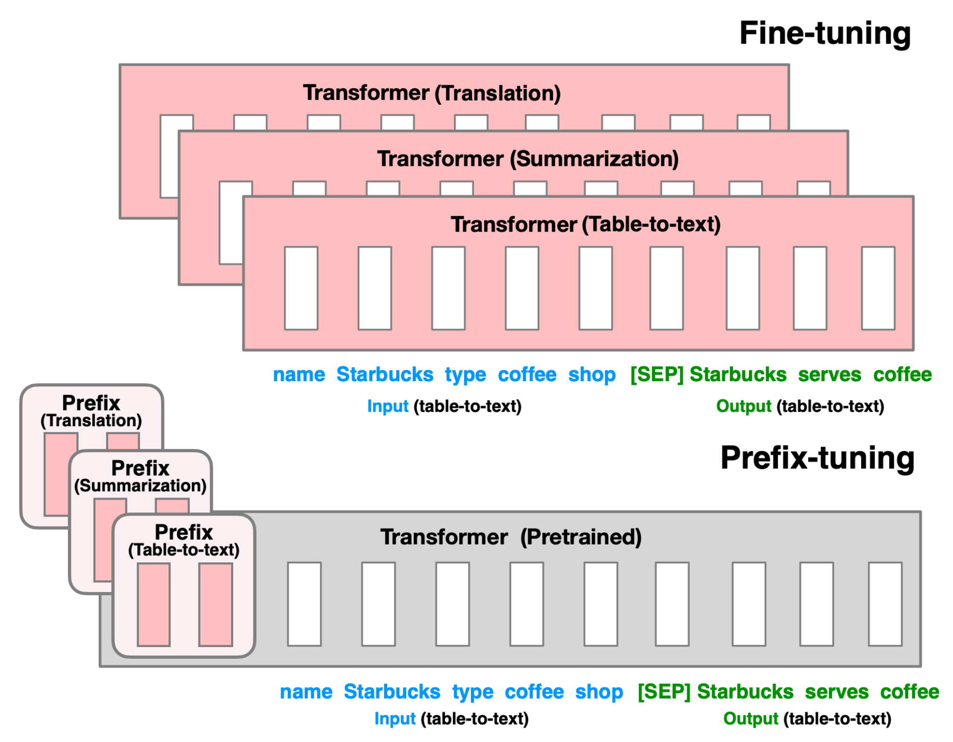
The prefix parameters are not tied to any embeddings associated with real words and are therefore more expressive for steering the context. Unfortunately, directly optimizing $P_\theta$ results in poor performance. To reduce the difficulty associated with high-dimensional training, the matrix $P_\theta$ is reparameterized using a smaller matrix $P’_\theta \in \mathbb{R}^{\vert\mathcal{P}_\text{idx}\vert \times c}$ and a large feed-forward network $\text{MLP}_\theta \in \mathbb{R}^{c\times \text{dim}(h_i)}$.

Performance improves with the prefix length $\vert\mathcal{P}_\text{idx}\vert$ up to a certain point, and this point varies across tasks.

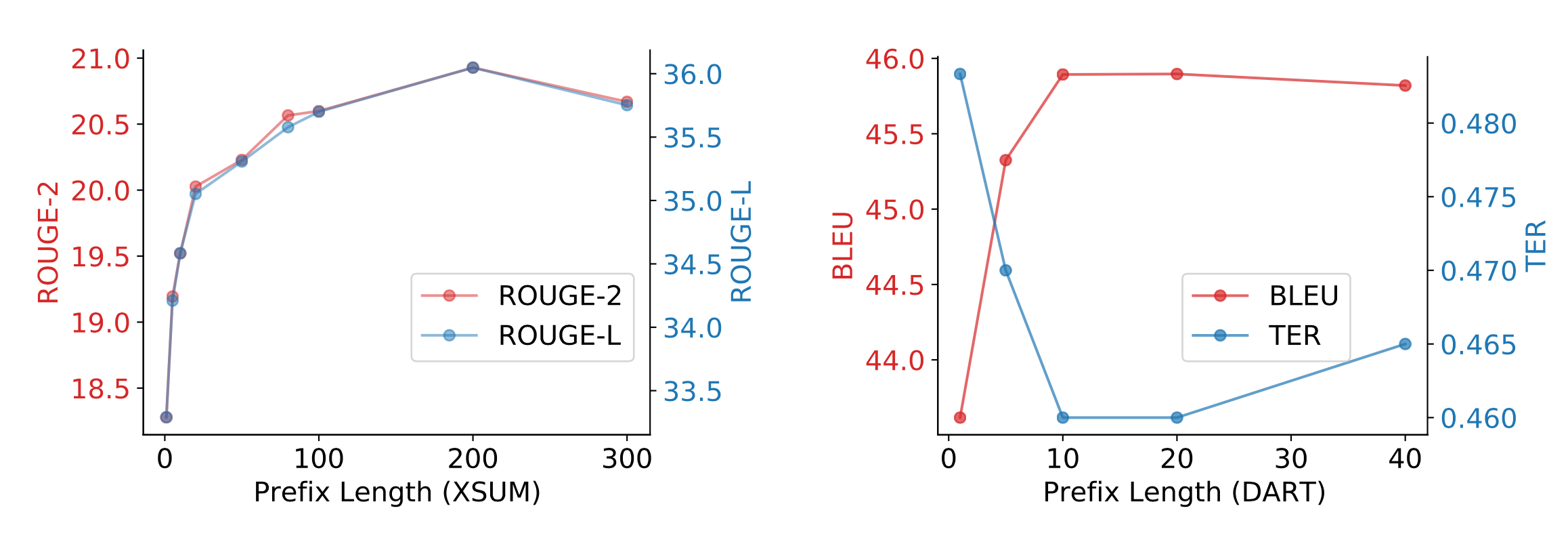
A few other noteworthy findings from their ablation studies include:

• Tuning only the embedding layer (without a prefix) is not sufficiently expressive.
• Placing the trainable parameter between $x$ and $y$, $[x; \text{INFIX}; y]$, slightly underperforms prefix-tuning, likely because it only affects the context for $y$, whereas the prefix affects both.
• Random initialization of $P_\theta$ yields low performance with high variance. In contrast, initializing $P_\theta$ with activations of real words improves generation, even if the words are irrelevant to the task.

Fine-tuned models achieve better task performance, but they can fail in low-data regimes. Both AutoPrompt and Prefix-Tuning were found to outperform fine-tuning when the training dataset is small (i.e., $10^2-10^3$ samples). As alternatives to fine-tuning, prompt design or learning the context embedding is much cheaper. AutoPrompt improves sentiment classification accuracy substantially more than manual prompts and achieves performance similar to linear probing. For the NLI task, AutoPrompt attains higher accuracy than linear probing. It can also retrieve facts more accurately than manual prompts. In low-data regimes, Prefix-Tuning achieves performance comparable to fine-tuning on table-to-text generation and summarization.

Two successive works, P-tuning (Liu et al. 2021; code) and Prompt Tuning (Lester et al. 2021), follow a similar idea of explicitly training continuous prompt embeddings, but with a few different choices regarding trainable parameters and architecture. Unlike Prefix-Tuning, which concatenates continuous prompt tokens at every hidden-state layer of the transformer, both P-tuning and Prompt Tuning non-invasively add continuous prompts only at the input to work effectively.

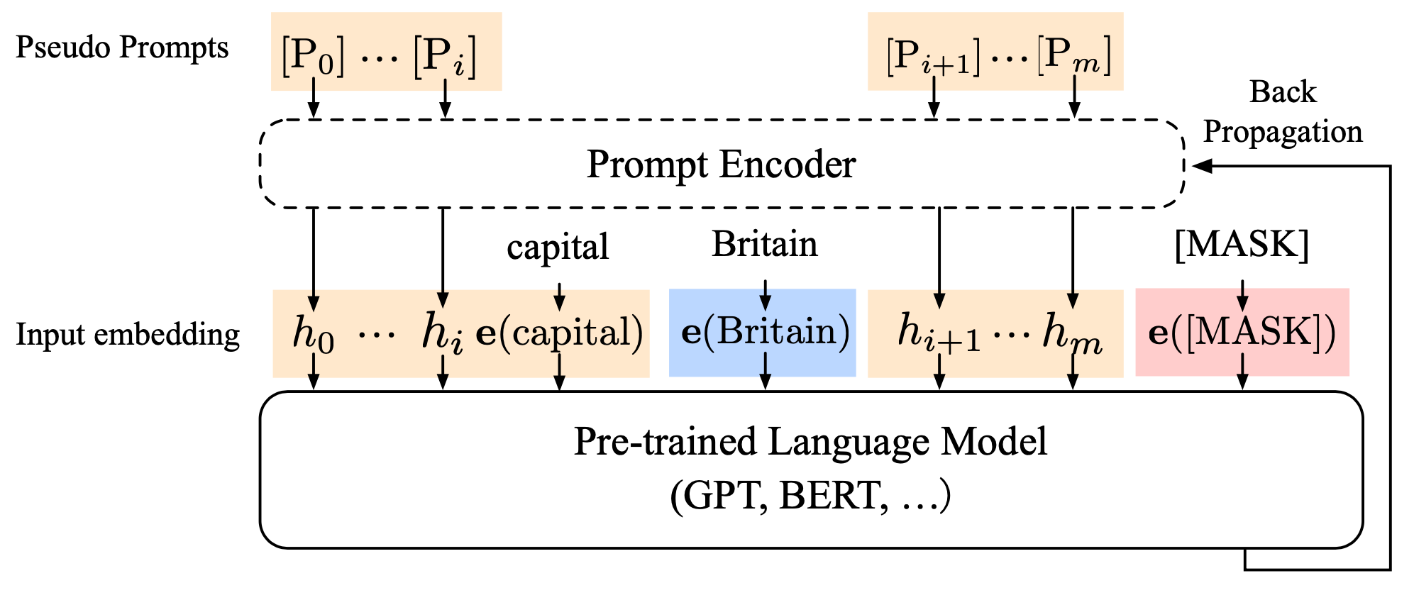
Let $[P_i]$ be the $i$-th token in the prompt template of P-tuning (Liu et al. 2021), we can denote a prompt as a sequence $T=\{[P_{0:i}], \mathbf{x}, [P_{i+1:m}], \mathbf{y}\}$. Each token $[P_i]$ does not have to be an actual token in the model vocabulary (a “pseudo-token”), and thus the encoded template $T^e$ looks as follows, and the pseudo-token hidden state can be optimized with gradient descent.

There are two major optimization challenges in P-tuning:

1. Discreteness: The word embeddings of a pretrained language model are highly discrete. It is difficult to optimize $h_i$ if they are initialized randomly.
2. Association: $h_i$ should depend on each other. Therefore, they develop a mechanism to model this dependency by training a lightweight LSTM-based prompt encoder:

P-tuning is more flexible than Prefix-Tuning, as it inserts trainable tokens in the middle of a prompt, not only at the beginning. The use of task-specific anchor tokens resembles combining manual prompt engineering with trainable prompts.

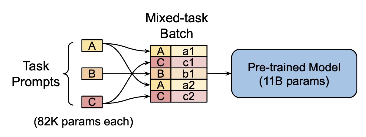
Prompt Tuning (Lester et al. 2021) largely simplifies the idea of Prefix-Tuning by allowing only an additional $k$ tunable tokens per downstream task to be prepended to the input text. The conditional generation is $p_{\theta, \theta_P}(Y \vert [P; X])$, where $P$ is the “pseudo prompt,” with parameters $\theta_P$ trainable via back-propagation. Both $X$ and $P$ are embedding vectors, and we have $X \in \mathbb{R}^{n \times d^e}, P \in \mathbb{R}^{k \times d^e}$ and $[P;X] \in \mathbb{R}^{(n+k) \times d^e}$, where $d^e$ is the dimensionality of the embedding space.

• Prompt tuning produces results that are competitive with model fine-tuning when the model becomes large (billions of parameters and above). This result is especially interesting given that large models are expensive to fine-tune and to run at inference time.
• With learned task-specific parameters, prompt tuning achieves better transfer learning when adapting to new domains. It outperforms fine-tuning on domain-shift problems.
• They also showed that prompt ensembling of multiple prompts for the same task yields further improvement.

The experiments investigated several prompt initialization schemes:

1. Random initialization by uniformly sampling from [-0.5, 0.5];
2. Sampling embeddings of the top 5000 common tokens;
3. Using the embedding values of the class label strings. If we do not have enough class labels to initialize the soft prompt, we fall back to scheme 2. Random initialization performs noticeably worse than the other two options.

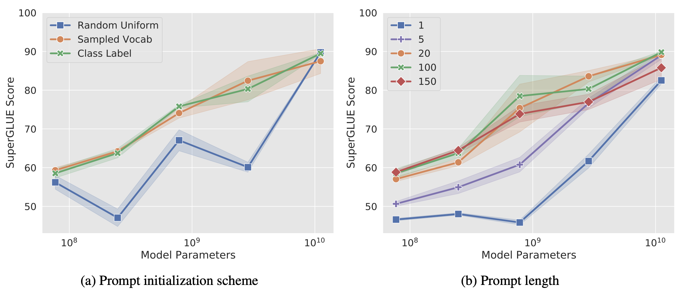
The pre-training objectives also have a major impact on the quality of prompt tuning. T5’s “span corruption” is not a good option here.

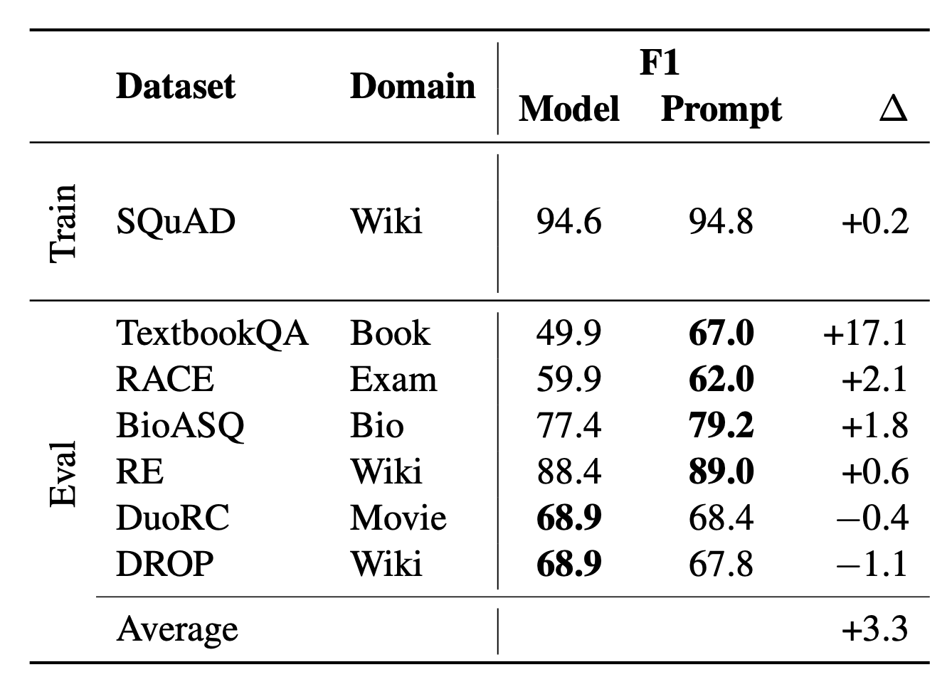
Prompt tuning is found to be less likely to overfit to a specific dataset. To evaluate robustness to the data-shift problem, they trained the model on one dataset for a task and evaluated it on the test dataset, but in a different domain. Prompt tuning is more resilient and can generalize better across domains.

Heuristic-based Search

Paraphrasing is a quick way to explore additional prompts similar to a known version, which can be done via back-translation. Using back-translation, the initial prompt is translated into $B$ candidates in another language, and then each is translated back into $B$ candidates in the original language. The resulting $B^2$ candidates are scored and ranked by their round-trip probabilities.

Ribeiro et al (2018) identified semantically equivalent adversaries (SEA) by generating a variety of paraphrases $\{x’\}$ of an input $x$ until it triggers a different prediction from the target function $f$:

where the score $p(x’\vert x)$ is proportional to translating $x$ into multiple languages and then translating it back into the original language.

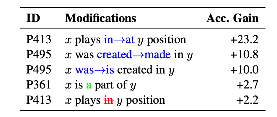
Examples of SEA rules include (What NOUN→Which NOUN), (WP is → WP’s’), (was→is), etc. They are considered “bugs” in the model. Applying these rules as data augmentation during model training helps make the model more robust and fix bugs.

Jiang et al (2020) attempts to validate whether a trained language model contains certain knowledge by automatically discovering better prompts to query it. This is within the scope of knowledge retrieval, where factual knowledge is represented as a triple $\langle x, r, y \rangle$ (subject, relation, object). Prompts can be mined from training sentences (e.g., Wikipedia descriptions) or expanded via paraphrasing.

Interestingly, small modifications to prompts can lead to large gains, as shown in Fig. X.

Fine-tuning

Fine-tuning is an intuitive way to guide an LM to produce desired content, commonly by training on supervised datasets or via RL. We can fine-tune all weights in the model or restrict fine-tuning to only the top or additional layers.

Conditional Training

Conditional training aims to learn a generative model conditioned on a control variable $z$, $p(y \vert x, z)$.

Fan et al (2018) trained a conditional language model for two-step story generation. First, a model outputs the story sketch, and then a story-writing model generates a story following that sketch. The conditioning mechanism on the sketch is implemented by a fusion model architecture. The fusion model enforces a form of residual learning that allows the story-writing model to focus on learning what the initial sketch generation model is missing. Also for story generation, Peng et al (2018) experimented with an ending valence-conditioned story generator LM, $p(x_t \vert x_{<t}, z)$, where $z$ is the label of the story ending (sad, happy, or neutral). Their language model is a bidirectional LSTM, and the label is mapped to a learned embedding that is then blended into the LSTM cell.

CTRL (Keskar et al., 2019; code) aims to train a language model conditioned on a control code $z$ using controllable datasets. CTRL learns the conditioned distribution $p(x \vert z)$ by training on raw text sequences with control code prefixes, such as [horror], [legal], etc. The learned model can then generate text according to the prompt prefix. The training data includes Wikipedia, OpenWebText, books, Amazon reviews, the Reddit corpus, and many more, where each dataset is assigned a control code, and each subreddit in the Reddit corpus has its own topic as a control code.

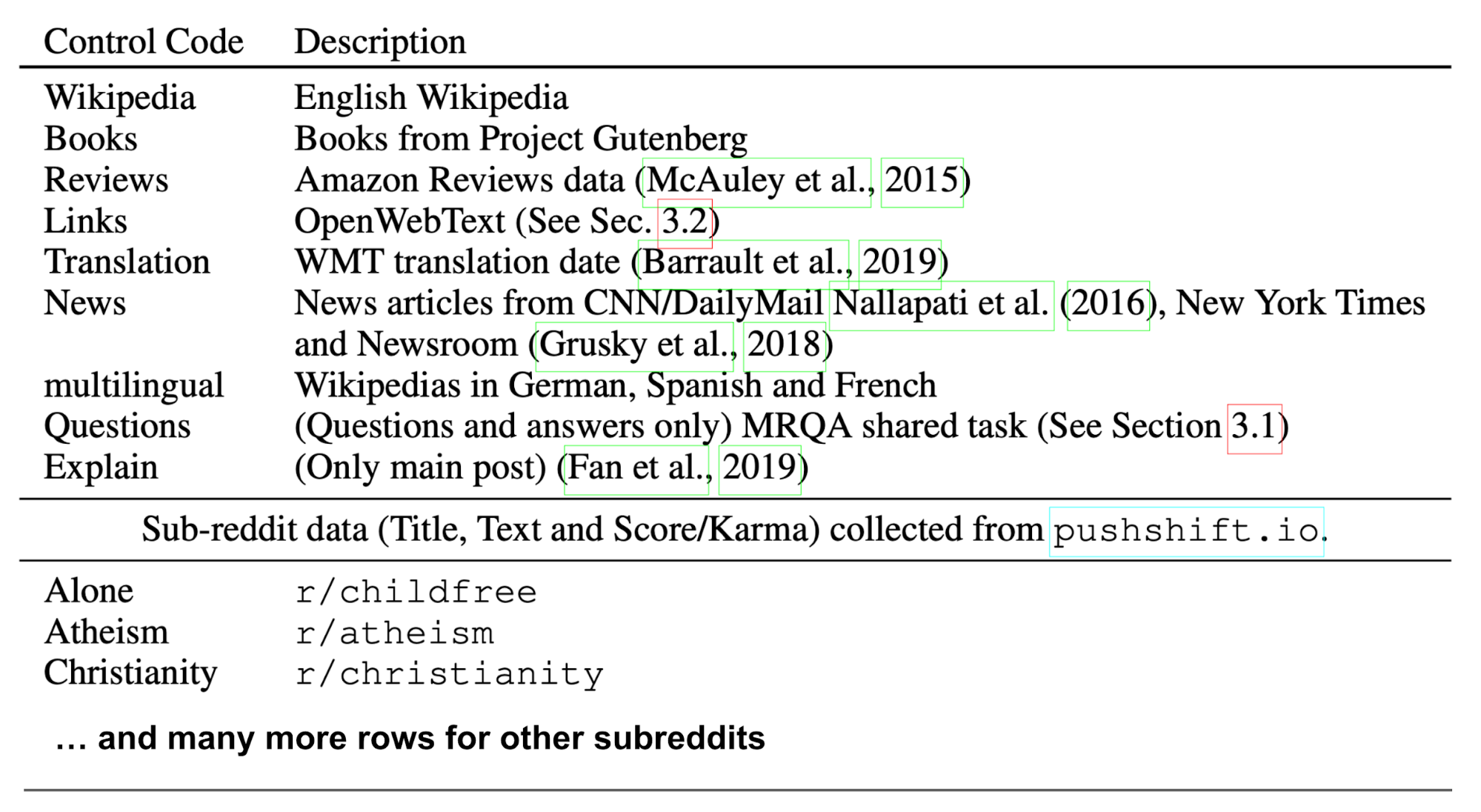
The control code can also be used for domain annotation of given tokens, because $p(z \vert x) \propto p(x \vert z) p(z)$, assuming a uniform prior over domains. One limitation of CTRL is the lack of control over what not to generate (e.g., avoiding toxicity).

Note that CTRL trains a transformer model from scratch. However, labeling all text within the same dataset with the same control code (e.g., all Wikipedia articles have “wikipedia” as the control code) feels quite constrained. Given that we often need highly customized control codes but only have a limited amount of labeled data, I would expect that fine-tuning an unconditional LM with a small labeled dataset, in the same way as CTRL, would work well too. However, how much data is needed and how good the sample quality might be are subject to experimentation.

RL Fine-tuning

Fine-tuning a sequential model with RL for an arbitrary, potentially non-differentiable reward function has been shown to work well for years (Ranzato et al., 2015). RL fine-tuning can address several issues with the teacher forcing method. With teacher forcing, the model minimizes a maximum-likelihood loss at each individual decoding step during training, but at test time it is asked to predict the entire sequence from scratch. This discrepancy between training and testing can lead to exposure bias and accumulated error. In contrast, RL fine-tuning can directly optimize task-specific, sequence-level metrics, such as BLEU for translation (Ranzato et al., 2015, Wu et al., 2016, Nguyen et al., 2017), ROUGE for summarization (Ranzato et al., 2015, Paulus et al., 2017, Wu and Hu, 2018), and customized metrics for story generation (Tambwekar et al., 2018).

Ranzato et al (2015) applied REINFORCE to train RNN models for sequence generation tasks. The model is first trained to predict the next token using cross-entropy loss (ML loss) and then alternately fine-tuned with both ML loss and REINFORCE (RL loss). During the second fine-tuning stage, the number of training steps for next-token prediction is gradually reduced to zero, and eventually only the RL loss is used. Experiments at the time showed that this sequence-level RL fine-tuning led to substantial improvements over several supervised-learning baselines.

Google implemented a similar approach in their neural machine translation system (Wu et al., 2016) and Paulus et al (2017) adopted this approach for the summarization task. The training objective contains two components: the ML loss for next-token prediction, $\mathcal{L}_\text{ML} = \sum_{(x, y^*)\sim\mathcal{D}} \log p_\theta(y^* \vert x)$, and the RL loss $\mathcal{L}_\text{RL}$ for maximizing the expected reward, where the reward per sequence is measured by BLEU or ROUGE. The model is first trained with $\mathcal{L}_\text{ML}$ until convergence and then fine-tuned with a linear combination of the two losses, $\mathcal{L}_\text{mix} = \alpha \mathcal{L}_\text{ML} + (1 - \alpha)\mathcal{L}_\text{RL}$.

The RL loss in Google NMT is to maximize the expected BLEU score:

where $y$ is the predicted sequence and $y^*$ is the ground truth.

Paulus et al (2017) added an additional weighting term based on the reward difference between two output sequences: $y$, sampled by drawing the next token according to the predicted probability, and $\hat{y}$, produced by greedily selecting the most likely token. This RL loss maximizes the conditional likelihood of the sampled sequence $y$ if it receives a higher reward than the greedy baseline $\hat{y}$:

RL Fine-tuning with Human Preferences

Reward learning is critical for capturing human preferences. Quantitative measures such as BLEU or ROUGE compute the overlap of words and n-gram phrases between sequences and do not always correlate with higher quality as judged by humans. Reward learning from human feedback (Christiano et al., 2017) is a better way to align what we measure with what we actually care about. Human feedback has been used to learn reward functions for applications such as story generation (Yi et al., 2019) and summarization (Böhm et al., 2019, Ziegler et al., 2019, Stiennon et al., 2020).

To generate more coherent conversation, Yi et al (2019) collected four types of binary human feedback for a conversation pair (user utterance, system response): whether the system response is (1) comprehensive, (2) on topic, (3) interesting, and (4) likely to lead to continuation of the conversation. An evaluator is trained to predict human feedback and is then used to rerank beam-search samples, to fine-tune the model, or to do both. (In fact, they did not use RL fine-tuning; instead, they used the evaluator to provide a discriminator loss in supervised fine-tuning.)

Let us define a learned reward function $R_\psi(x, y)$, parameterized by $\psi$, as a measure of the quality of output $y$ given input $x$.

To learn the ground-truth reward $R^*$ defined by human judgments, Böhm et al (2019) compared two loss functions:

(1) Regression loss: simply minimizing the mean squared error.

(2) Preference loss: learning to agree with the ground-truth reward,

Their experiments showed that the preference loss achieves the best performance, where the reward model is a thin MLP layer on top of BERT sentence embeddings.

Ziegler et al (2019) collected human labels by asking annotators to select the best candidate $y_b$ from a few options $\{y_i\}$ given an input $x \sim \mathcal{D}$. The candidates are sampled as $y_0, y_1 \sim p(.\vert x)$ and $y_2, y_3 \sim \pi(.\vert x)$. We should note that human labeling can exhibit very high disagreement when the ground truth is ambiguous.

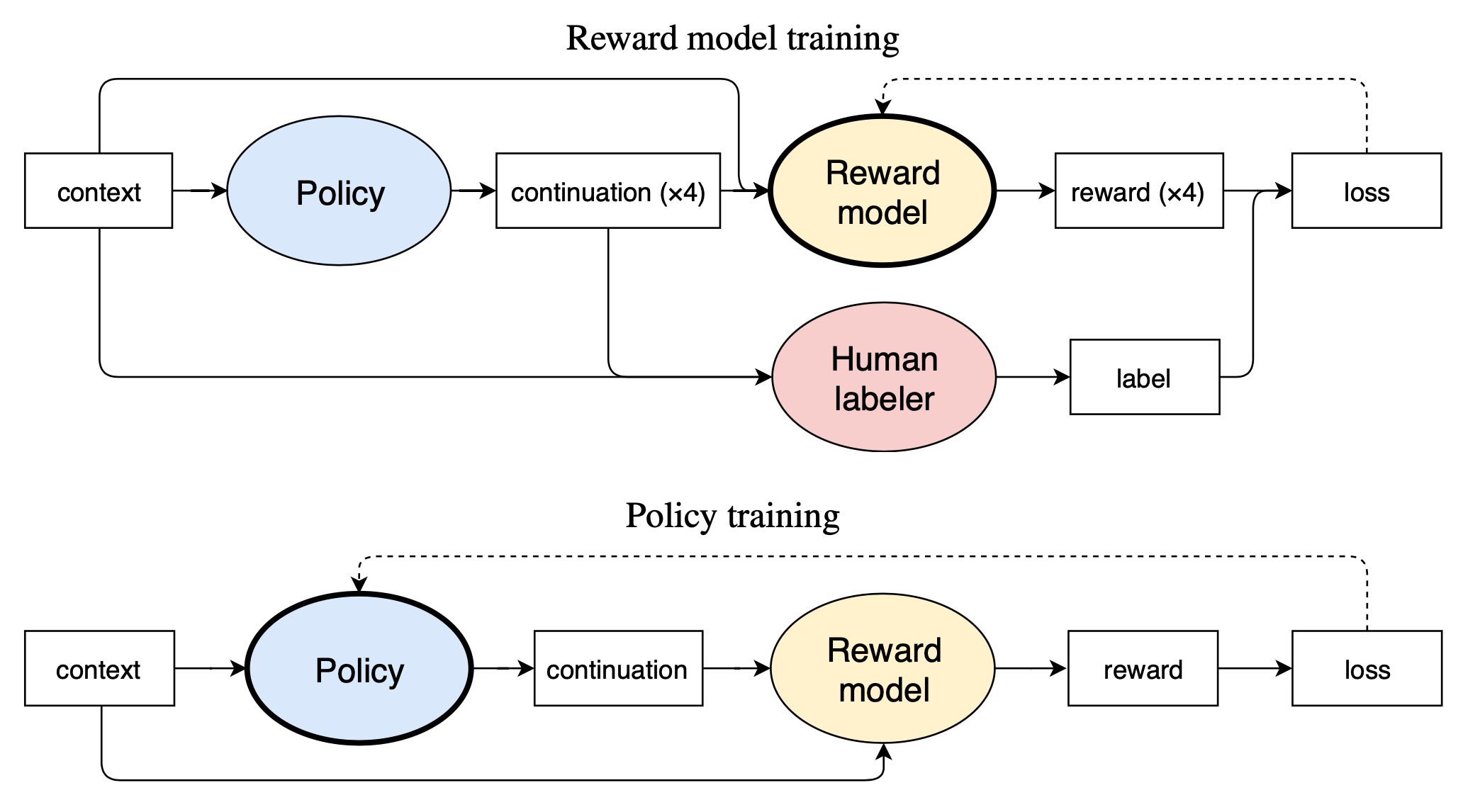
The reward model is implemented as a pretrained language model with an additional randomly initialized linear layer on top of the final embedding output. It is trained to minimize the loss:

To keep the scale consistent during training, the reward model is normalized to have mean 0 and variance 1.

During RL fine-tuning, the policy $\pi$, initialized from a pretrained language model $p$, is optimized via PPO with the learned reward model above. To prevent the policy from deviating too far from its original behavior, a KL penalty is added:

When running online data collection, the human labeling process continues during RL fine-tuning, so labelers can review results generated by the latest policy. The number of human labels is distributed evenly throughout training. Meanwhile, the reward model is periodically retrained. Online data collection turned out to be important for the summarization task but not for the text-continuation task. In their experiments, jointly training the reward model and the policy with shared parameters did not work well and can lead to overfitting due to the large imbalance between dataset sizes.

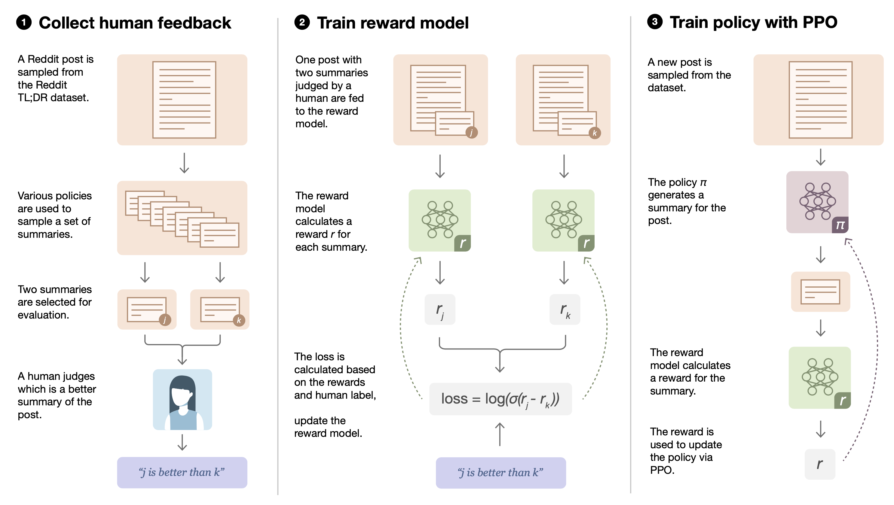
In the following work (Stiennon et al., 2020), human label collection was further simplified to selecting the better option from a pair of summaries, $y_b \in\{y_0, y_1\}$. The reward model loss was updated to optimize the log-odds of the selected summary:

Guided Fine-tuning with a Steerable Layer

Instead of fine-tuning the entire model, fine-tuning only a small additional set of parameters while keeping the base model fixed is computationally cheaper.

In computer vision, plug-and-play generative networks (PPGN; Nguyen et al., 2017) generate images with different attributes by plugging a discriminator $p(a \vert x)$ into a base generative model $p(x)$. Then, a sample with a desired attribute $a$ can be drawn from $p(x \vert a) \propto p(a \vert x)p(x)$. Inspired by PPGN, the plug-and-play language model (PPLM; Dathathri et al., 2019) combines one or more simple attribute models with a pretrained language model for controllable text generation.

Given an attribute $a$ and a generated sample $x$, let an attribute model be $p(a\vert x)$. To control content generation, the current latent representation at time $t$, $H_t$ (containing a list of key-value pairs per layer), can be shifted by $\Delta H_t$ in the direction of the sum of two gradients:

• One gradient increases the log-likelihood of attribute $a$ under $p(a \vert x)$, so the output content acquires the desired attribute.
• The other increases the log-likelihood under the unmodified language model $p(x)$, so the generated text remains fluent and smooth natural language.

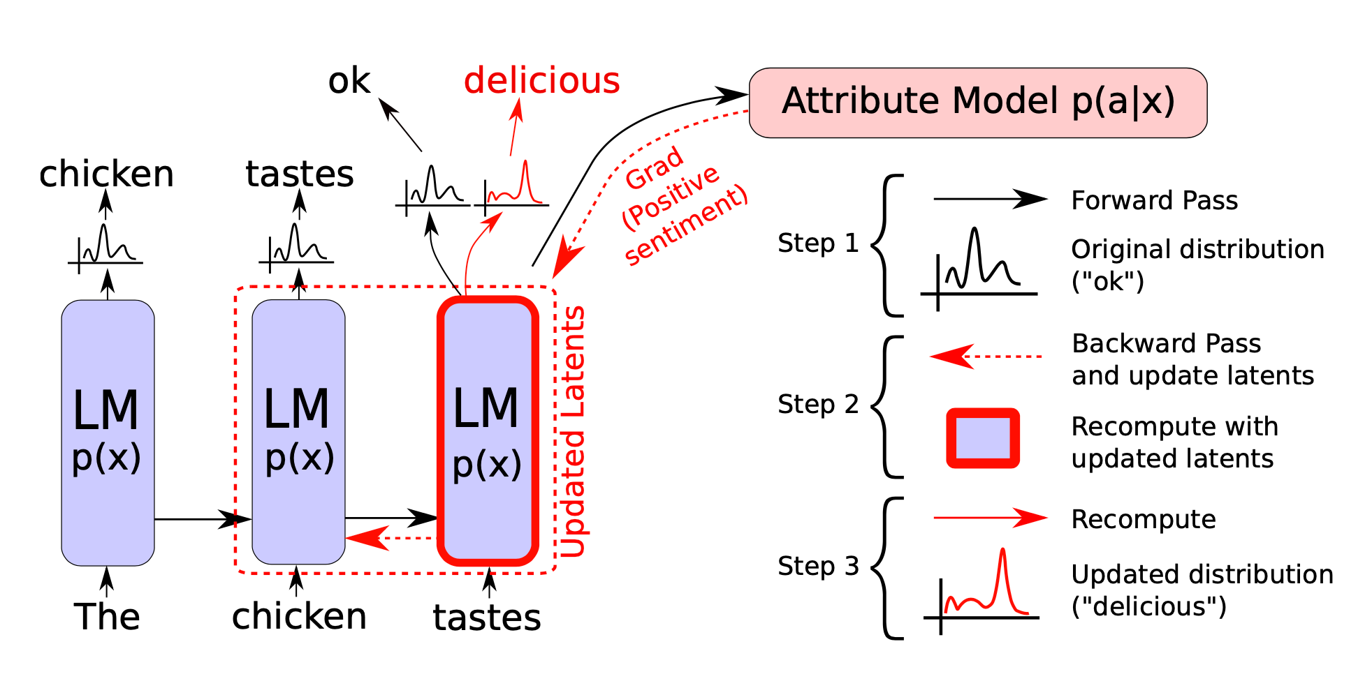
To shift the output at decoding time, PPLM performs three passes in total: one forward pass, one backward pass, and one forward pass:

1. First, a forward pass is performed to compute the likelihood of attribute $a$ via $p(a\vert x)$;
2. Let $\Delta H_t$ be a stepwise update to the hidden state $H_t$ such that $(H_t + \Delta H_t)$ shifts the distribution of generated text toward having attribute $a$. $\Delta H_t$ is initialized to zero. Then, a backward pass updates the LM hidden states using normalized gradients from the attribute model $\nabla_{\Delta H_t} \log p(a \vert H_t + \Delta H_t)$ as

where $\gamma$ is a normalization scaling coefficient, set per layer, and $\alpha$ is the step size. This update can be repeated $m \in [3, 10]$ times 3. The final forward pass recomputes a new distribution over the vocabulary from the updated latents $\tilde{H}_t = H_t + \Delta H_t$. The next token is sampled from the updated distribution.

Multiple attribute models can be mixed and matched during generation with customized weights, acting as a set of “control knobs.” The PPLM paper explored two types of attribute models:

1. The simplest attribute model is based on a predefined bag of words (BoW), $\{w_1, \dots, w_k\}$, that specifies a topic of interest.
   

To encourage the model to output the desired words at least once, but not at every step, they normalize the gradient by the maximum gradient norm.
Interestingly, they found that increasing the probability of generating words in the bag also increases the probability of generating related but not identical words on the same topic. 2. The discriminator attribute models are based on learned classifiers that define preferences via a distribution rather than hard samples.

To ensure language fluency, PPLM applied two additional design choices:

1. Minimizing the KL divergence between the modified and unmodified LM, as commonly seen in other RL fine-tuning approaches (see above).
2. It performs post-norm fusion to continuously tie the generated text to the unconditional LM $p(x)$, $x_{t+1} \sim \frac{1}{\beta}(\tilde{p}_{t+1}^{\gamma_\text{gm}} p_{t+1}^{1-\gamma_\text{gm}})$, where $p_{t+1}$ and $\tilde{p}_{t+1}$ are the unmodified and modified output distributions, respectively. $\beta$ is a normalizing factor. $\gamma_\text{gm} \in [0.8, 0.95]$ balances between predictions from the pre- and post-modification models.

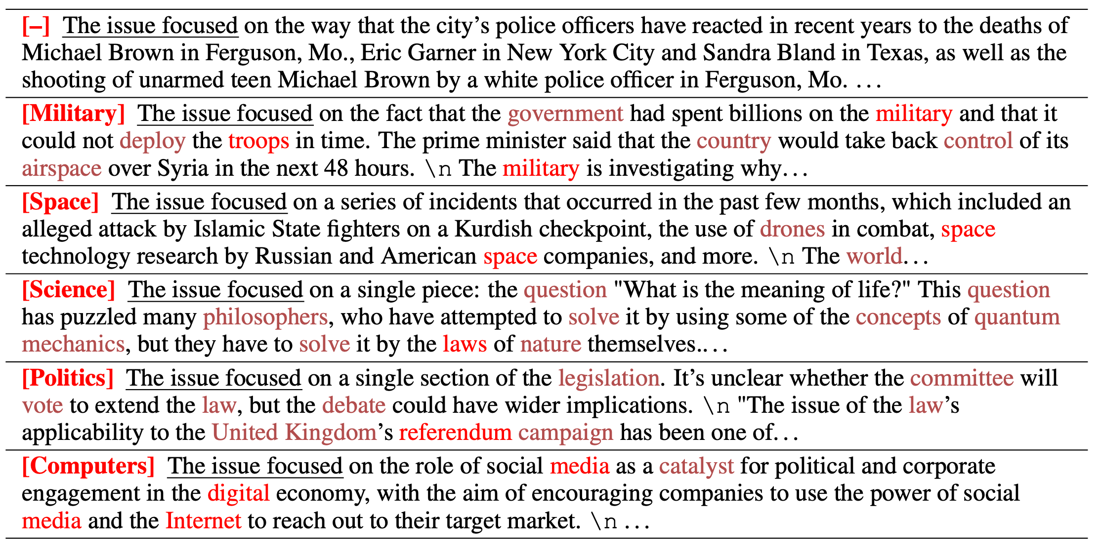
Interestingly, they found substantial variance in the degree of controllability across topics. Some topics (religion, science, politics) are easier to control than others (computers, space).

One clear drawback of PPLM is that, due to multiple passes at every decoding step, test-time computation becomes much more expensive.

Similar to PPLM, DELOREAN (DEcoding for nonmonotonic LOgical REAsoNing; Qin et al., 2020) incorporates future context via backpropagation. Given input text $\mathbf{x}$, DELOREAN aims to generate a continuation $\mathbf{y} = [y_1, \dots, y_N]$ such that $y$ satisfies certain constraints defined by a context $z$. To keep generation differentiable, a soft representation of $y$ is tracked: $\tilde{\mathbf{y}}=(\tilde{y}_1, \dots, \tilde{y}_N)$, where $\tilde{y}_i \in \mathbb{R}^V$ are logits over the vocabulary. $\tilde{\mathbf{y}}^{(t)}$ is the soft representation at iteration $t$.

Given the representation $\tilde{y}^{(t-1)}$ at iteration $t$, it runs the following procedures:

1. Backward: The constraint is represented as a loss function $\mathcal{L}(\mathbf{x}, \tilde{\mathbf{y}}^{(t-1)}, z))$. The logits are updated via gradient descent: $\tilde{y}^{(t), b}_n = \tilde{y}_n^{(t-1)} - \lambda \nabla_{\tilde{y}_n} \mathcal{L}(\mathbf{x}, \tilde{\mathbf{y}}^{(t-1)}, z)$.
2. Forward: Run a forward pass to ensure the generated text is fluent. $\tilde{y}^{(t),f}_n = \text{LM}(\mathbf{x}, \tilde{\mathbf{y}}^{(t)}_{1:n-1})$.
3. Then, linearly combine the two logits to create a new representation: $\tilde{y}^{(t)}_n = \gamma \tilde{y}^{(t), f}_n + (1-\gamma) \tilde{y}^{(t), b}_n$. Note that each $\tilde{y}^{(t)}_n$ is needed to sample the next $\tilde{y}^{(t),f}_{n+1}$.

Side-tuning (Zhang et al., 2019) trains a lightweight side network that learns a residual on top of the original model outputs without modifying the pretrained model weights. Unlike PPLM, no gradient update is applied to the hidden states. It is a simple yet effective approach for incremental learning. The base model is treated as a black-box model and does not necessarily need to be a neural network. The side-tuning setup assumes that the base and side models are fed exactly the same input, and the side model is learned independently.

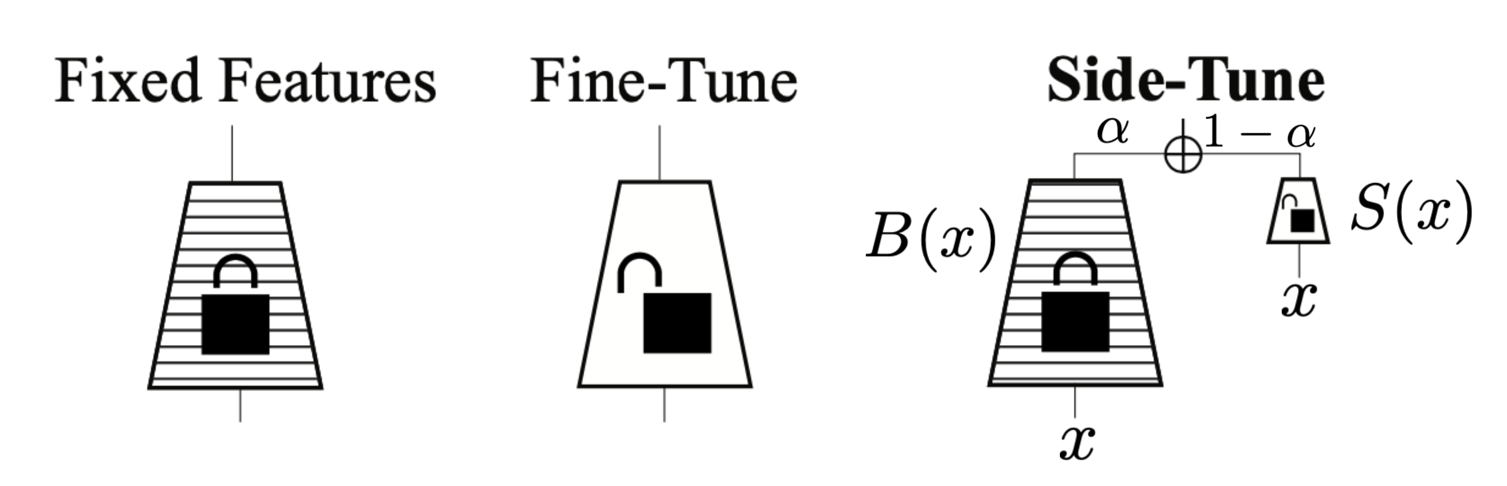
The paper explored different strategies for fusing predictions from the base and side models: product is the worst, while sum ($\alpha$-blending), MLP, and FiLM are comparable. Side-tuning can achieve better performance when it is trained with intermediate amounts of data and when the base network is large.

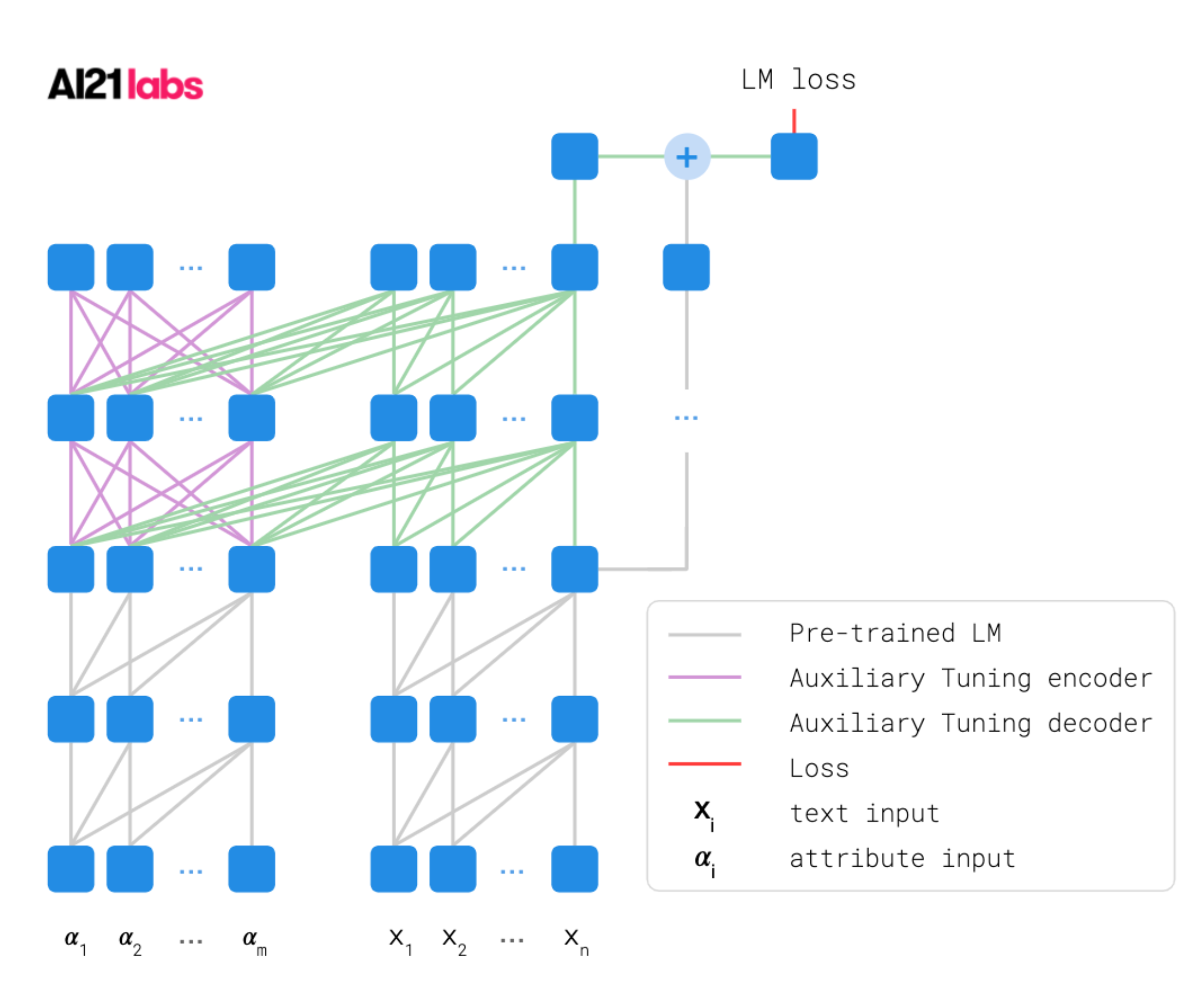
Auxiliary tuning (Zeldes et al., 2020) augments the original pretrained model with an auxiliary model that shifts the output distribution according to the target task. The base and auxiliary model outputs are merged at the logits level. The combined model is trained to maximize the likelihood $p(x_t\vert x_{<t}, z)$ of the target output.

The conditional probability $p(x_t\vert x_{<t}, z)$ can be decomposed into two parts:

1. $p(x_t\vert x_{<t})$ assigns high probabilities to fluent token sequences;
2. a shift of $p(x_t\vert x_{<t})$ toward $p(x_t\vert x_{<t}, z)$.

By Bayes' rule, we have

Therefore, the auxiliary model $\text{logits}_\text{aux}(x_t \vert x_{<t}, z))$ should effectively learn to predict $p(z \vert x_{\leq t})$. In the experiments of Zeldes et al., 2020, the auxiliary model can reuse the intermediate layers of the pretrained LM for feature extraction.

GeDi (Kruse et al., 2020) guides text generation via a Generative Discriminator. The discriminator is implemented as a class-conditional language model (CC-LM), $p_\theta(x_{1:t} \vert z)$. The discriminator guides generation at each decoding step by computing classification probabilities for all possible next tokens via Bayes' rule, by normalizing over two contrastive class-conditional distributions:

1. One is conditioned on the control code $z$ for the desired attribute.
2. The other is conditioned on the anti-control code $\bar{z}$ for undesired attributes.

GeDi relies on the contrast between $p_\theta(x_{1:t} \vert z)$ and $p_\theta(x_{1:t} \vert \bar{z})$ to compute the probability that the sequence belongs to the desired class. The discriminator loss is to maximize the probability of the desired attribute $z$:

where $p(z) = \exp(b_z) / \sum_{z’} \exp(b_{z’})$ and $b_z$ is a learned class prior. The probabilities are normalized by the current sequence length $\tau$ to make generation robust for sequences of variable lengths. $\tau_i$ is the sequence length of the $i$-th input $x^{(i)}$ in the dataset.

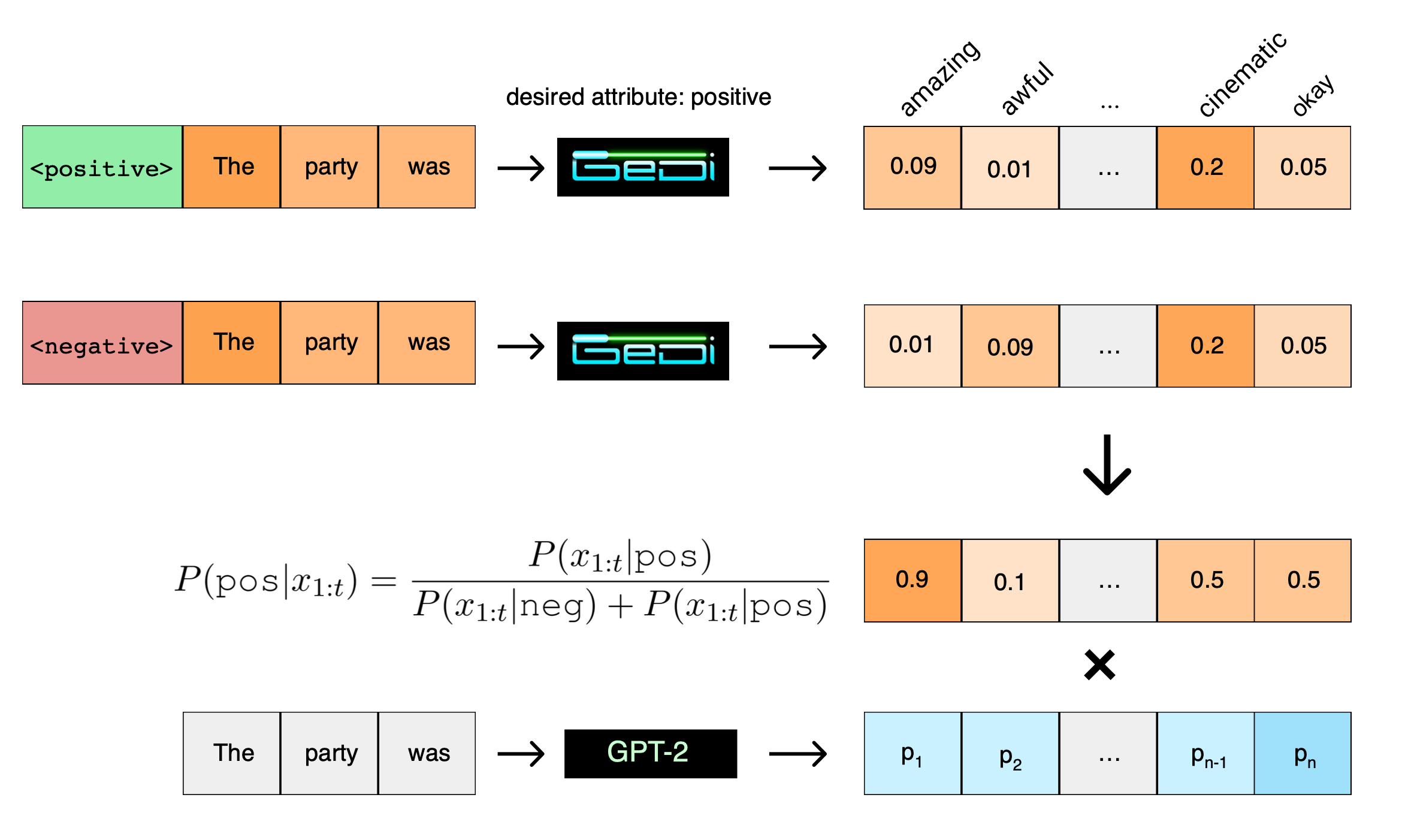
They fine-tuned a GPT2-medium model with a control code, similar to how CTRL is trained, to form a CC-LM using a linear combination of discriminative loss and generative loss. This discriminator model is then used as GiDe to guide generation by a larger language model, such as GPT2-XL.

One way to decode with GeDi is to sample from a weighted posterior $p^w(x_{t+1}\vert x_{1:t}, z) \propto p(z \vert x_{1:t+1})^w p(x_{t+1} \vert x_{1:t})$, where $w>1$ applies additional bias toward the desired class $z$. In the sampling process, only tokens with class or next-token probability greater than a certain threshold are selected.

GeDi-guided generation in their experiments showed strong controllability and ran 30x faster than PPLM.

Distributional Approach

Generation with Distributional Control (GDC; Khalifa, et al. 2020) frames controlled text generation as the optimization of a probability distribution subject to a constraint. It involves two major steps.

Step 1: Learn an EBM of the target model

Let’s denote a pretrained LM as $a$ and a target LM with desired features as $p$. The desired features can be defined by a set of predefined real-valued feature functions $\phi_i(x), i=1,\dots,k$ over $x \in X$, denoted as a vector $\boldsymbol{\phi}$. When sequences $x \in X$ are sampled according to the desired model $p$, the feature expectations $\mathbb{E}_{x\sim p}\boldsymbol{\phi}(x)$ should be close to $\bar{\boldsymbol{\mu}}$, referred to as “moment constraints”. The feature function $\phi_i$ can take discrete values (e.g., an identity function for a binary classifier) or continuous probabilities. Meanwhile, the fine-tuned model $p$ should not diverge too much from $a$ by maintaining a small KL divergence measure.

In summary, given a pretrained model $a$, we would like to find a target model $p$ such that:

where $\mathcal{C}$ is the set of all distributions over $X$ that satisfy the moment constraints.

According to theorems in information geometry, $p$ can be approximated by an EBM (energy-based model, an unnormalized probability distribution) $P$ in exponential form, such that $p(x) \propto P(x)$ and $p(x)=\frac{1}{Z}P(x)$, where $Z=\sum_x P(x)$. The energy-based model can be approximated by:

Let’s define importance weight $w(x, \boldsymbol{\lambda}) = \frac{P(x)}{a(x)} = \exp\langle\boldsymbol{\lambda}\cdot\boldsymbol{\phi}(x)\rangle$. Given a large number of sequences sampled from the pretrained model $x_1, \dots, x_N \sim a(x)$,

Using SGD on the objective $|\boldsymbol{\mu}(\boldsymbol{\lambda}) - \bar{\boldsymbol{\mu}}|^2_2$, we can obtain an estimated value for $\boldsymbol{\lambda}$ and a representation of $P(x)=a(x)\exp\langle\boldsymbol{\lambda}\cdot\boldsymbol{\phi}(x)\rangle$. $P(x)$ is a sequential EBM because $a$ is an autoregressive model.

Step 2: Learn the target probability distribution

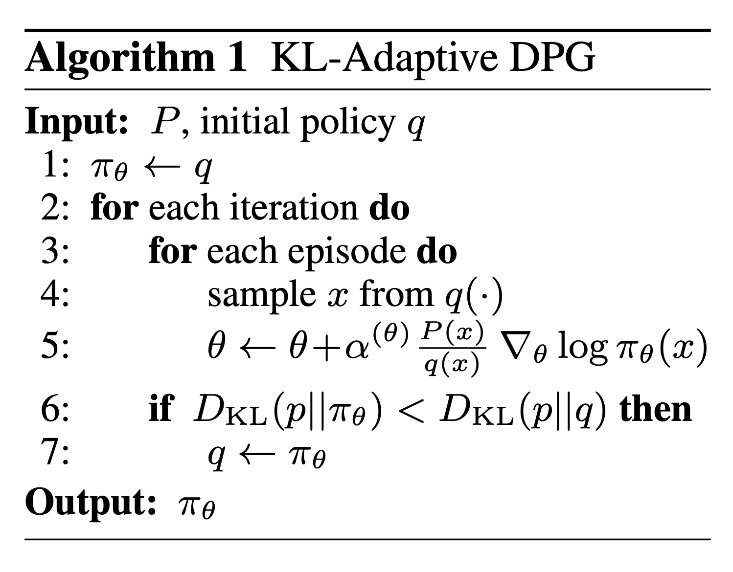
The EBM $P(x)$ can compute ratios of probabilities for two sequences, but it cannot sample from $p(x)$ without knowing $Z$. To sample from a sequential EBM, the paper proposed using Distributional Policy Gradient (DPG; but not this DPG) with the objective of obtaining an autoregressive policy $\pi_\theta$ to approximate a target distribution $p$ by minimizing the cross-entropy $H(p, \pi_\theta)$. DPG proceeds through a sequence of iterations. Within each iteration, the proposed distribution $q$ is used for sampling, and we can also correct the cross-entropy loss with importance weights:

To learn such a $\pi_\theta$, the paper adopts a KL-adaptive version of DPG: It updates $q$ only when the estimated policy $\pi_\theta$ moves closer to $p$. This adaptive step is important for fast convergence.

This approach can be used to model various constraints in controllable text generation:

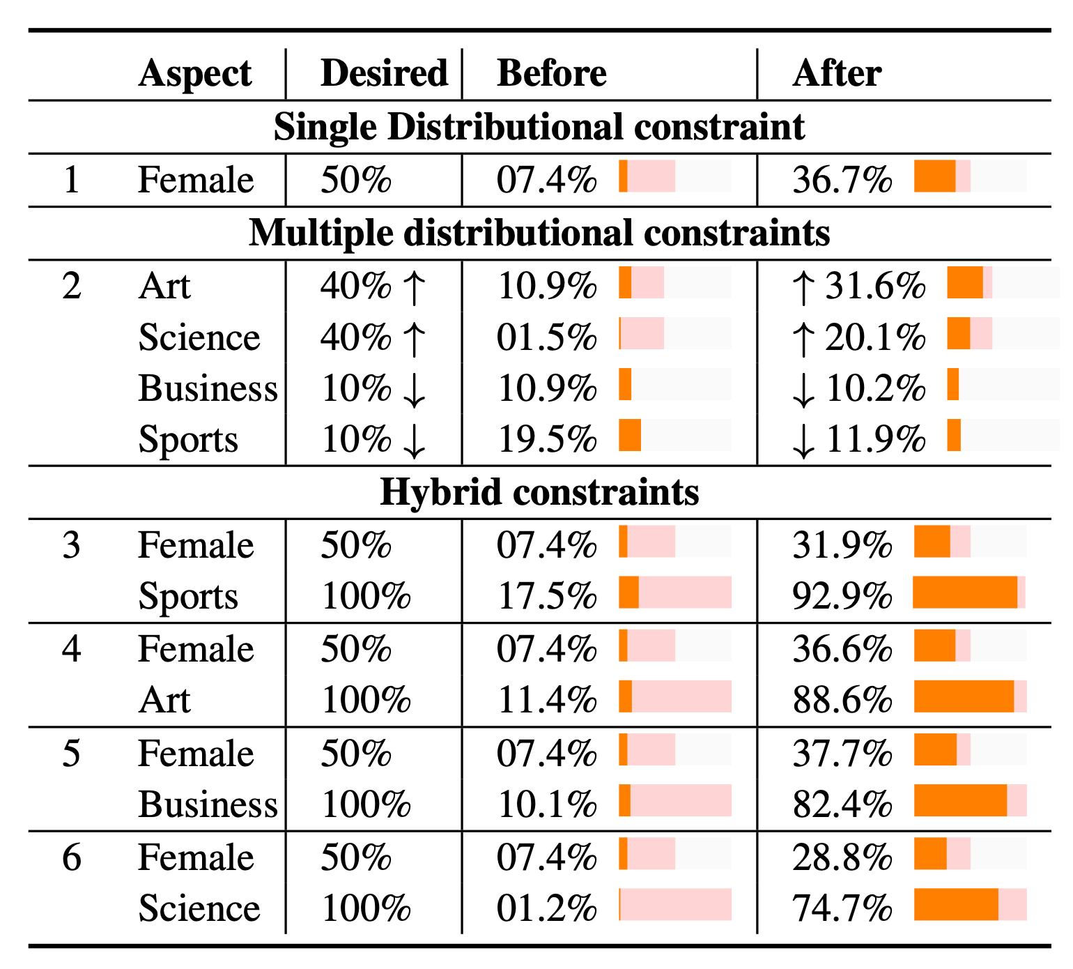
1. Pointwise constraints: $\phi_i$ is a binary feature, such as constraining the presence or absence of words, or classifier-based constraints.
2. Distributional constraints: $\phi_i$ represents a probability distribution, such as constraining the probability of gender, topic, etc. Their experiments showed substantial progress in debiasing a GPT-2 model trained on the Wikipedia Biographies corpus. The percentage of generated biographies about females increased from 7.4% to 35.6%.
3. Hybrid constraints: Combine multiple constraints by simply summing them.

Compared to other baselines, GDC with pointwise constraints diverges less from the base model $a$ and produces smoother curves.

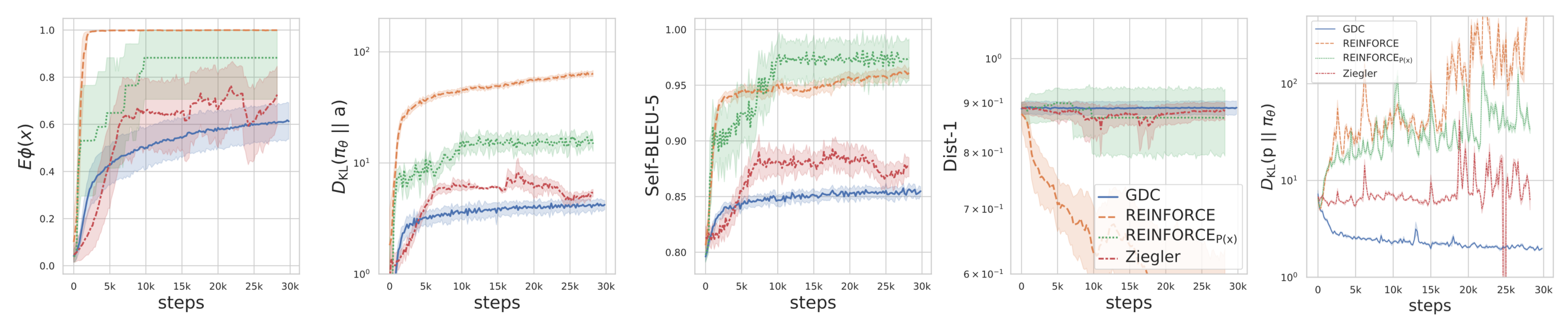
• REINFORCE that optimizes the reward $\phi$ directly ($\text{REINFORCE}$ in Fig. X.) without constraints converges quickly but deviates substantially from the original model.
• REINFORCE that optimizes $P(x)$ ($\text{REINFORCE}_{P(x)}$ in Fig. X.) has low sample diversity.
• Compared to Ziegler et al., 2019 GDC has smoother learning curves and produces a richer vocabulary.

Unlikelihood Training

The standard approach of maximizing the log-likelihood loss in language model training leads to incorrect token distribution, which cannot be addressed using only clever decoding methods. Such models tend to output high-frequency words too often and low-frequency words too rarely, especially when using deterministic decoding (e.g., greedy or beam search). In other words, they are overconfident in their predictions.

Unlikelihood training (Welleck & Kulikov et al. 2019] seeks to address this by directly incorporating a preference against unwanted content into the training objective. It combines two updates:

• A standard maximum-likelihood update to assign high probability to true tokens;
• A new type of unlikelihood update to avoid assigning high probability to unwanted tokens.

Given a token sequence $(x_1, \dots, x_T)$ and a set of negative candidate tokens $\mathcal{C}^t = \{c_1, \dots , c_m\}$ at step $t$, where each token $x_i, c_j \in \mathcal{V}$, the combined loss for step $t$ is defined as:

One approach for constructing $\mathcal{C}^t$ is to randomly select candidates from model-generated sequences.

Unlikelihood training can be extended to the sequence-level, where the negative continuation is defined by a sequence of per-step negative candidate sets. These should be designed to penalize properties we do not want. For example, we can penalize repeating n-grams as follows:

Their experiments used unlikelihood training to avoid repetition in language model outputs and showed better results, with less repetition and more unique tokens, compared to standard MLE training.

Citation

Cited as:

Weng, Lilian. (Jan 2021). Controllable neural text generation. Lil’Log. https://lilianweng.github.io/posts/2021-01-02-controllable-text-generation/.

Or

@article{weng2021conditional,
  title   = "Controllable Neural Text Generation.",
  author  = "Weng, Lilian",
  journal = "lilianweng.github.io",
  year    = "2021",
  month   = "Jan",
  url     = "https://lilianweng.github.io/posts/2021-01-02-controllable-text-generation/"
}

References

[1] Patrick von Platen. “How to generate text: using different decoding methods for language generation with Transformers” Hugging Face blog, March 18, 2020.

[2] Angela Fan, et al. “Hierarchical Neural Story Generation/” arXiv preprint arXiv:1805.04833 (2018).

[3] Ari Holtzman et al. “The Curious Case of Neural Text Degeneration.” ICLR 2020.

[4] Marjan Ghazvininejad et al. “Hafez: an interactive poetry generation system.” ACL 2017.

[5] Ari Holtzman et al. “Learning to write with cooperative discriminators.” ACL 2018.

[6] Ashutosh Baheti et al. “Generating More Interesting Responses in Neural Conversation Models with Distributional Constraints.” EMNLP 2018.

[7] Jiatao Gu et al. “Trainable greedy decoding for neural machine translation.” EMNLP 2017.

[8] Kyunghyun Cho. “Noisy Parallel Approximate Decoding for Conditional Recurrent Language Model.” arXiv preprint arXiv:1605.03835. (2016).

[9] Marco Tulio Ribeiro et al. “Semantically equivalent adversarial rules for debugging NLP models.” ACL 2018.

[10] Eric Wallace et al. “Universal Adversarial Triggers for Attacking and Analyzing NLP.” EMNLP 2019. [code]

[11] Taylor Shin et al. “AutoPrompt: Eliciting Knowledge from Language Models with Automatically Generated Prompts.” EMNLP 2020. [code]

[12] Zhengbao Jiang et al. “How Can We Know What Language Models Know?” TACL 2020.

[13] Nanyun Peng et al. “Towards Controllable Story Generation.” NAACL 2018.

[14] Nitish Shirish Keskar, et al. “CTRL: A Conditional Transformer Language Model for Controllable Generation” arXiv preprint arXiv:1909.05858 (2019).[code]

[15] Marc’Aurelio Ranzato et al. “Sequence Level Training with Recurrent Neural Networks.” ICLR 2016.

[16] Yonghui Wu et al. “Google’s Neural Machine Translation System: Bridging the Gap between Human and Machine Translation.” CoRR 2016.

[17] Romain Paulus et al. “A Deep Reinforced Model for Abstractive Summarization.” ICLR 2018.

[18] Paul Christiano et al. “Deep Reinforcement Learning from Human Preferences.” NIPS 2017.

[19] Sanghyun Yi et al. “Towards coherent and engaging spoken dialog response generation using automatic conversation evaluators.” INLG 2019.

[20] Florian Böhm et al. “Better rewards yield better summaries: Learning to summarise without references.” EMNLP 2019. [code]

[21] Daniel M Ziegler et al. “Fine-tuning language models from human preferences.” arXiv preprint arXiv:1909.08593 (2019). [code]

[22] Nisan Stiennon, et al. “Learning to summarize from human feedback.” arXiv preprint arXiv:2009.01325 (2020).

[23] Sumanth Dathathri et al. “Plug and play language models: a simple approach to controlled text generation.” ICLR 2020. [code]

[24] Jeffrey O Zhang et al. “Side-tuning: Network adaptation via additive side networks” ECCV 2020.

[25] Ben Kruse et al. “GeDi: Generative Discriminator Guided Sequence Generation.” arXiv preprint arXiv:2009.06367.

[26] Yoel Zeldes et al. “Technical Report: Auxiliary Tuning and its Application to Conditional Text Generatio.” arXiv preprint arXiv:2006.16823.

[27] Thomas Scialom, et al. “Discriminative Adversarial Search for Abstractive Summarization” ICML 2020.

[28] Clara Meister, et al. “If beam search is the answer, what was the question?” EMNLP 2020.

[29] Xiang Lisa Li and Percy Liang. “Prefix-Tuning: Optimizing Continuous Prompts for Generation.” arXiv preprint arXiv:2101.00190 (2021).

[30] Lianhui Qin, et al. “Back to the Future: Unsupervised Backprop-based Decoding for Counterfactual and Abductive Commonsense Reasoning.” arXiv preprint arXiv:2010.05906 (2020).

[31] Muhammad Khalifa, et al. “A Distributional Approach to Controlled Text Generation” Accepted by ICLR 2021.

[32] Aditya Grover, et al. “Bias correction of learned generative models using likelihood-free importance weighting.” NeuriPS 2019.

[33] Yuntian Deng et al. “Residual Energy-Based Models for Text Generation.” ICLR 2020.

[34] Brian Lester et al. “The Power of Scale for Parameter-Efficient Prompt Tuning.” arXiv preprint arXiv:2104.08691 (2021).

[35] Xiao Liu et al. “GPT Understands, Too.” arXiv preprint arXiv:2103.10385 (2021).

[36] Welleck & Kulikov et al. “Neural Text Generation with Unlikelihood Training” arXiv:1908.04319 (2019).