[Updated on 2022-03-13: add expert choice routing.]
[Updated on 2022-06-10]: Greg and I wrote a shorted and upgraded version of this post, published on OpenAI Blog: “Techniques for Training Large Neural Networks”

In recent years, larger pre-trained language models have delivered improved results on many NLP benchmark tasks. Training large and deep neural networks remains challenging because it demands significant GPU memory and extended training time.

At the same time, the memory capacity of an individual GPU worker is limited, and many modern large models have grown beyond what fits on a single GPU. To address this, a number of parallelism paradigms enable training across multiple GPUs, complemented by architecture and memory-saving designs that help make training very large neural networks practical.

Training Parallelism

The primary bottleneck in training very large neural network models is the heavy demand for GPU memory, far exceeding what a single GPU machine can host. Beyond the model weights themselves (for example, tens of billions of floating-point values), storing intermediate computation results, such as gradients and optimizer states (for example, momentums and variations in Adam), is often even more costly. In addition, large models are typically paired with large training corpora, so a single process may take an impractically long time to finish.

For these reasons, parallelism becomes essential. Parallelism can be applied along multiple dimensions, including data, model architecture, and tensor operations.

Data Parallelism

The most straightforward form of data parallelism (DP) replicates the same model weights across multiple workers and assigns each worker a fraction of the data to process concurrently.

Naive DP performs poorly when the model itself is larger than a single GPU node’s memory. Approaches such as GeePS (Cui et al. 2016) address this by offloading parameters that are temporarily unused back to the CPU, enabling training with limited GPU memory even when the model does not fit on one machine. The parameter swapping should occur in the background and should not disrupt the training computation.

After each minibatch, workers must synchronize gradients or weights to prevent staleness. Two primary synchronization strategies are common, each with clear advantages and disadvantages:

1. Bulk synchronous parallels (BSP): Workers synchronize at the end of every minibatch. This avoids stale model weights and yields strong learning efficiency, but each machine must pause and wait for others to send gradients.
2. Asynchronous parallel (ASP): Each GPU worker processes data asynchronously, without waiting or stalling. However, this can easily result in stale weights and therefore reduced statistical learning efficiency. Even if it increases raw computation throughput, it may not reduce the time to convergence.

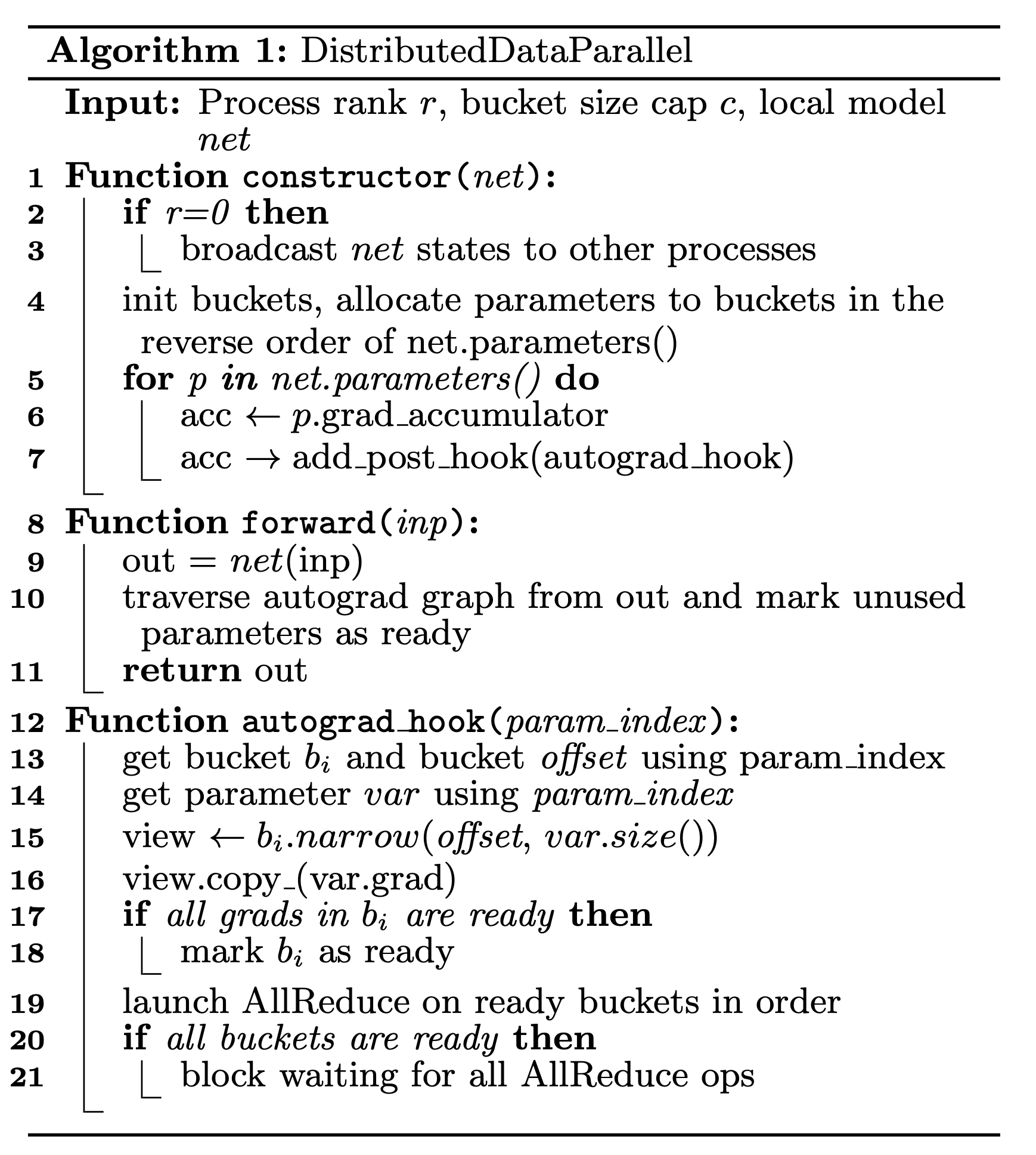
An intermediate option is to synchronize gradients globally once every $x$ iterations ($x > 1$). In PyTorch, this is called “gradient accumulation” in Distribution Data Parallel (DDP) starting in v1.5 (Li et al. 2021). Gradient bucketing avoids immediate AllReduce operations by grouping multiple gradients into a single AllReduce, improving throughput. Computation and communication scheduling can also be optimized using the computation graph.

Model Parallelism

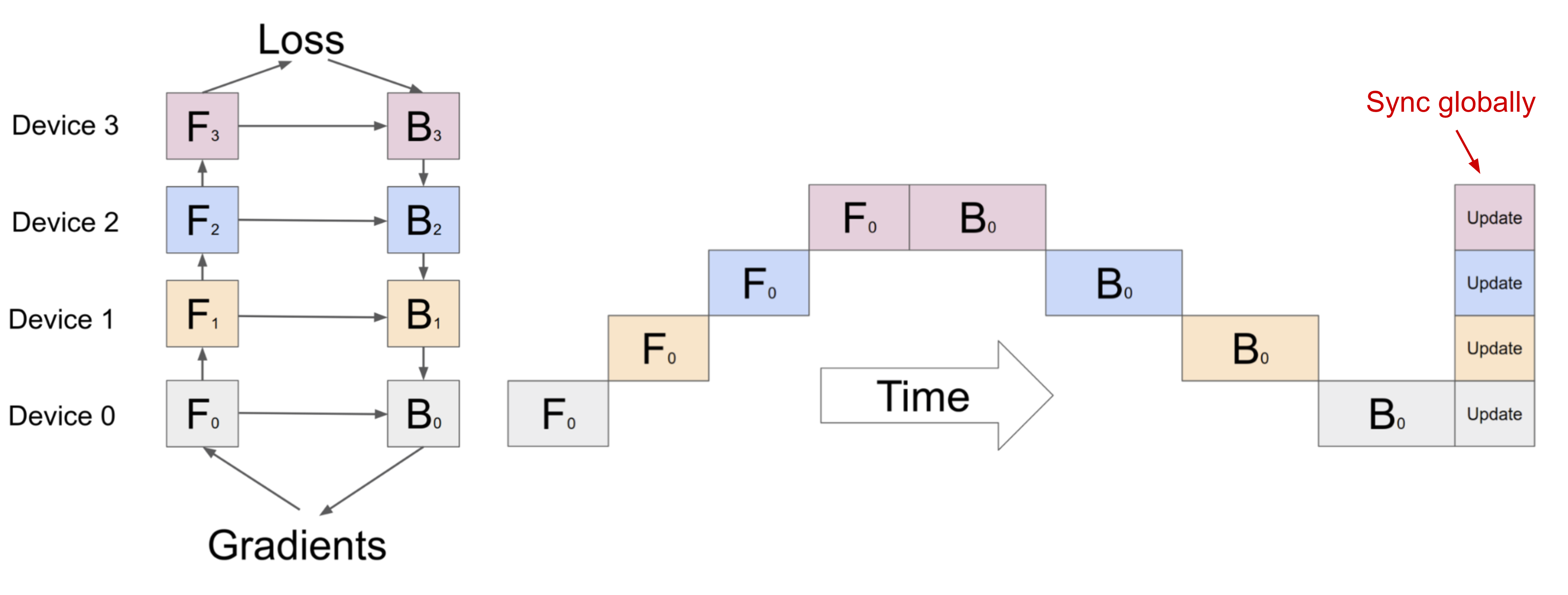
Model parallelism (MP) targets situations where model weights cannot fit on a single node. Under MP, computation and parameters are partitioned across multiple machines. Unlike data parallelism, where every worker holds a full copy of the model, MP assigns only a fraction of the parameters to each worker, reducing both memory usage and per-worker computation.

Because deep neural networks are often built as a vertical stack of layers, a natural approach is to split a large model by layer, grouping a small, consecutive set of layers into one partition on a worker. However, a naive implementation that runs each data batch through the workers sequentially creates large bubbles of idle time due to sequential dependencies, leading to substantial under-utilization of compute resources.

Pipeline Parallelism

Pipeline parallelism (PP) blends model parallelism with data parallelism to reduce inefficient “bubbles” of idle time. The central idea is to split a minibatch into multiple microbatches so that each pipeline stage can process a microbatch concurrently. Note that every microbatch requires two passes, a forward pass and a backward pass. Inter-worker communication transfers activations during the forward pass and gradients during the backward pass. Different methods vary in how they schedule these passes and how they aggregate gradients. The number of partitions (workers) is also referred to as the pipeline depth.

In GPipe (Huang et al. 2019), gradients from multiple microbatches are aggregated and applied synchronously at the end of the batch. This synchronous gradient descent preserves learning consistency and efficiency regardless of the number of workers. As illustrated in Fig. 3, bubbles still occur, but they are substantially smaller than in naive model parallelism. Given $m$ evenly split microbatches and $d$ partitions, and assuming each microbatch forward and backward pass takes one unit of time, the bubble fraction is:

The GPipe paper reports that bubble overhead is nearly negligible when the number of microbatches exceeds 4x the number of partitions $m > 4d$ (when activation recomputation is used).

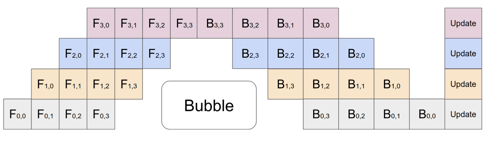
GPipe can achieve almost linear throughput speedup as the number of devices increases, although this is not guaranteed when model parameters are unevenly distributed across workers.

PipeDream (Narayanan et al. 2019) schedules each worker to alternate between forward and backward computation using the 1F1B pattern. In PipeDream terminology, each model partition is a “stage,” and each stage worker may have multiple replicas to run data parallelism. PipeDream uses a deterministic round-robin load-balancing strategy to distribute work across stage replicas, ensuring that the forward and backward passes for the same minibatch execute on the same replica.

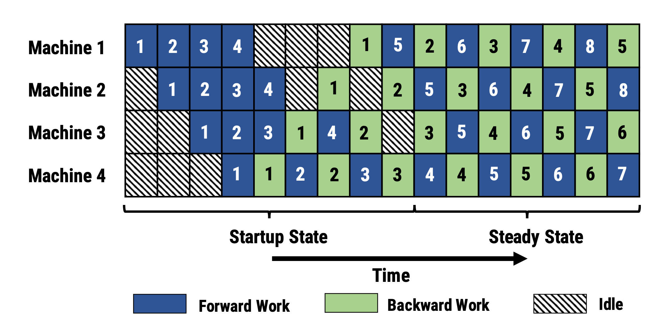
Because PipeDream does not perform an end-of-batch global gradient synchronization across all workers, a naive 1F1B implementation can easily cause the forward and backward passes of a microbatch to use different versions of the model weights, reducing learning efficiency. PipeDream introduces several mechanisms to mitigate this:

• Weight stashing: Each worker tracks multiple versions of the model weights, ensuring that the same weight version is used for both forward and backward passes for a given data batch.
• Vertical sync (Optional): Weight versions flow between stages alongside activations and gradients. Computation then uses the corresponding stashed version propagated from the previous stage, maintaining version consistency across workers. Note that this is asynchronous, unlike GPipe.

At the start of training, PipeDream profiles per-layer compute time and memory cost, then solves for an optimized partitioning of layers into stages via dynamic programming.

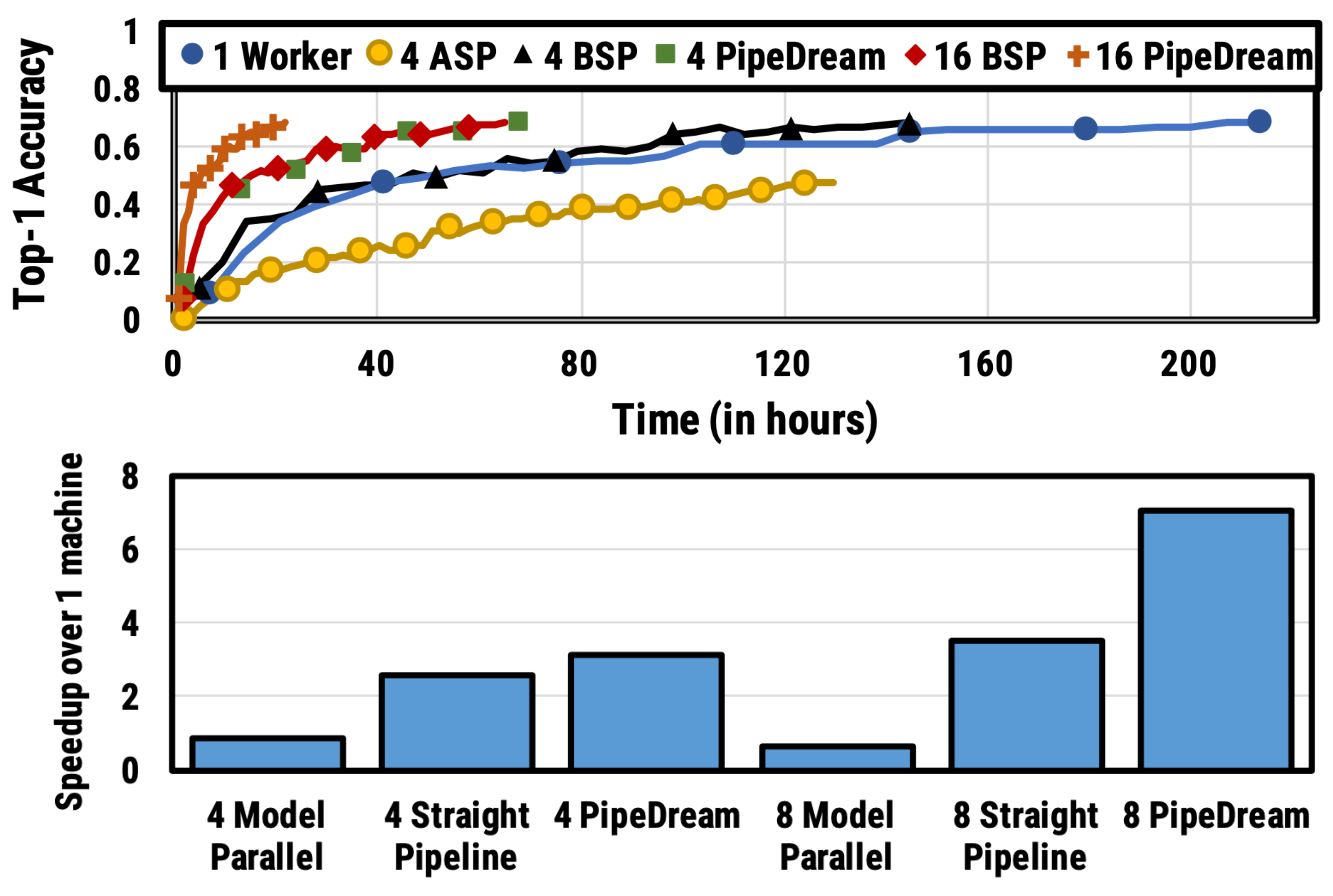
Two later variants of PipeDream reduce the memory cost associated with stashed weight versions (Narayanan et al. 2021).

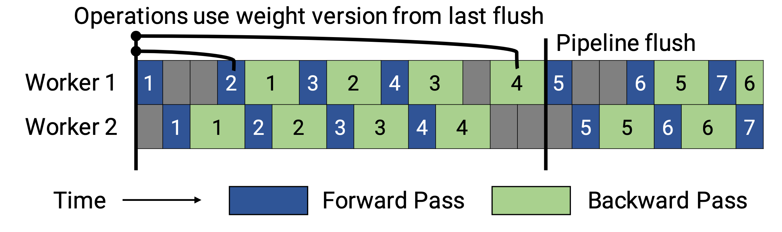
PipeDream-flush periodically performs a globally synchronized pipeline flush, similar to GPipe. This substantially reduces memory footprint (that is, it maintains only a single version of the model weights) at the cost of a small throughput reduction.

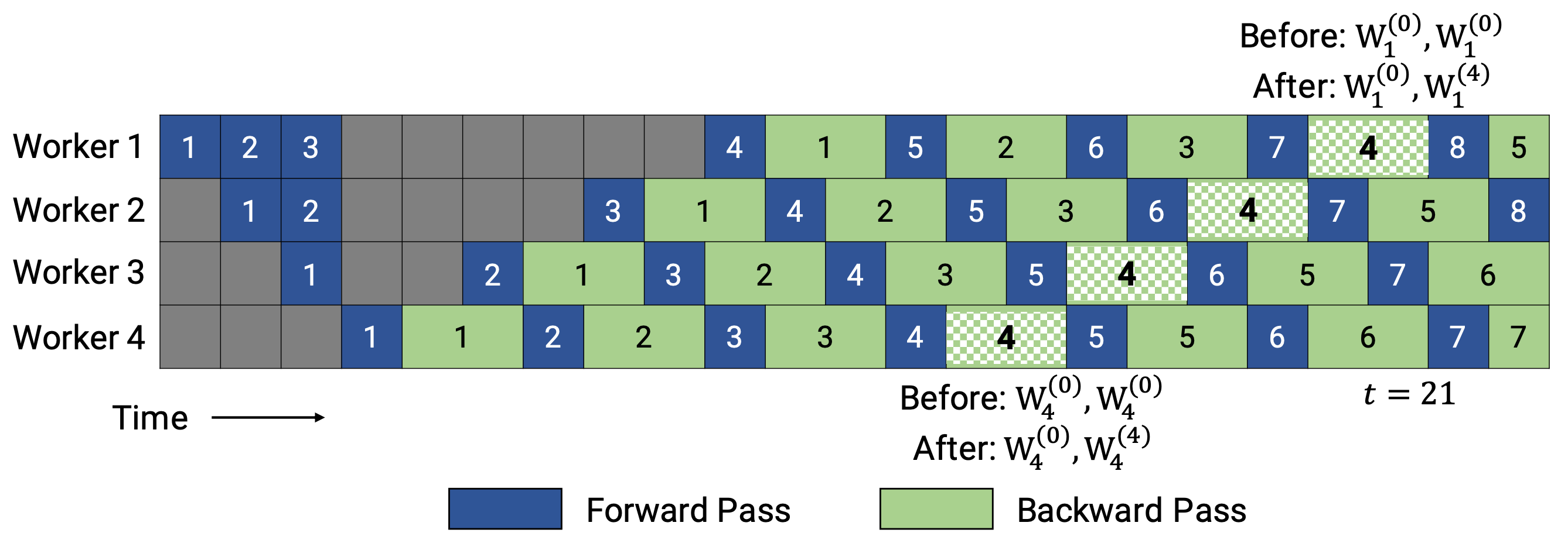
PipeDream-2BW keeps only two versions of model weights, where “2BW” stands for “double-buffered weights.” It produces a new model version every $k$ microbatches, and $k$ must be larger than the pipeline depth $d$, $k > d$. A freshly updated version cannot immediately replace the previous one, because some remaining backward passes still depend on the older version. Overall, only two versions are stored, significantly reducing memory usage.

Tensor Parallelism

Model parallelism and pipeline parallelism both partition a model vertically. In contrast, we can also partition the computation of a single tensor operation horizontally across multiple devices. This is known as tensor parallelism (TP).

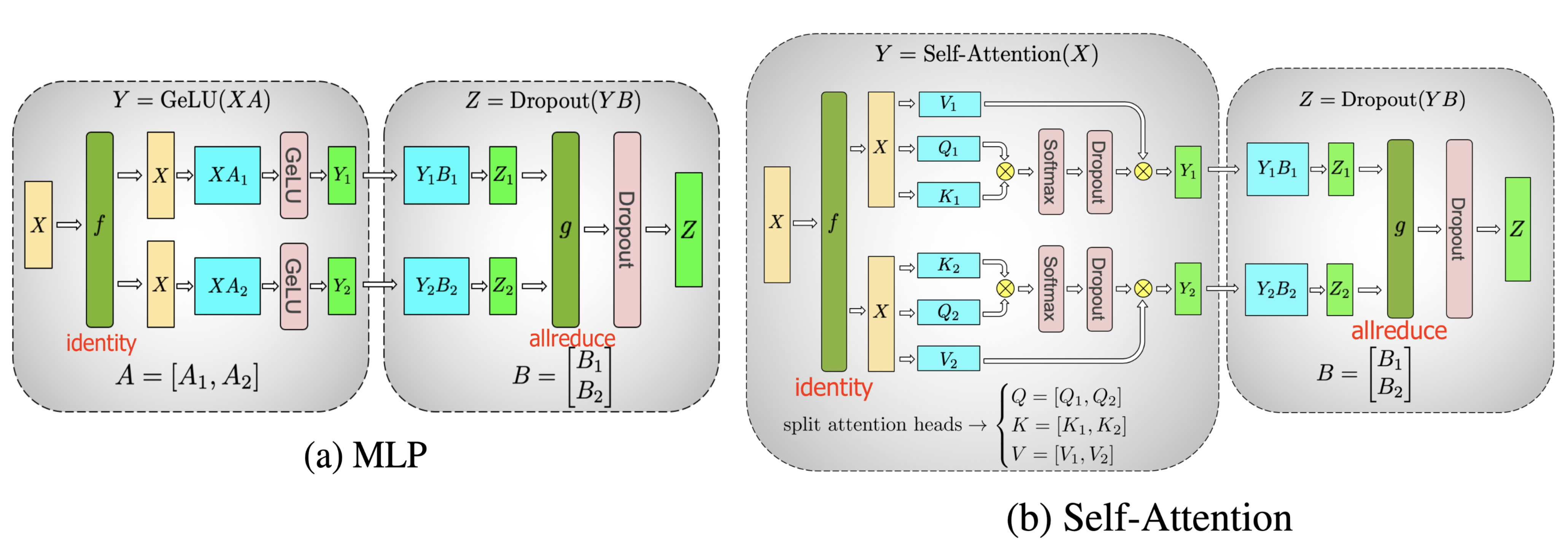
Given the popularity of transformers, consider a transformer as a representative example. A transformer primarily consists of MLP blocks and self-attention blocks. Megatron-LM (Shoeybi et al. 2020) proposes a simple approach for parallelizing intra-layer computation in both MLP and self-attention.

An MLP layer in a transformer includes a GEMM (general matrix multiply) followed by a non-linear GeLU transform. Split the weight matrix $A$ by columns:

For self-attention, the block performs GEMMs with the query ($Q$), key ($K$), and value weights ($V$) in parallel according to the same partitioning, and then combines the results with another GEMM to produce the attention head outputs.

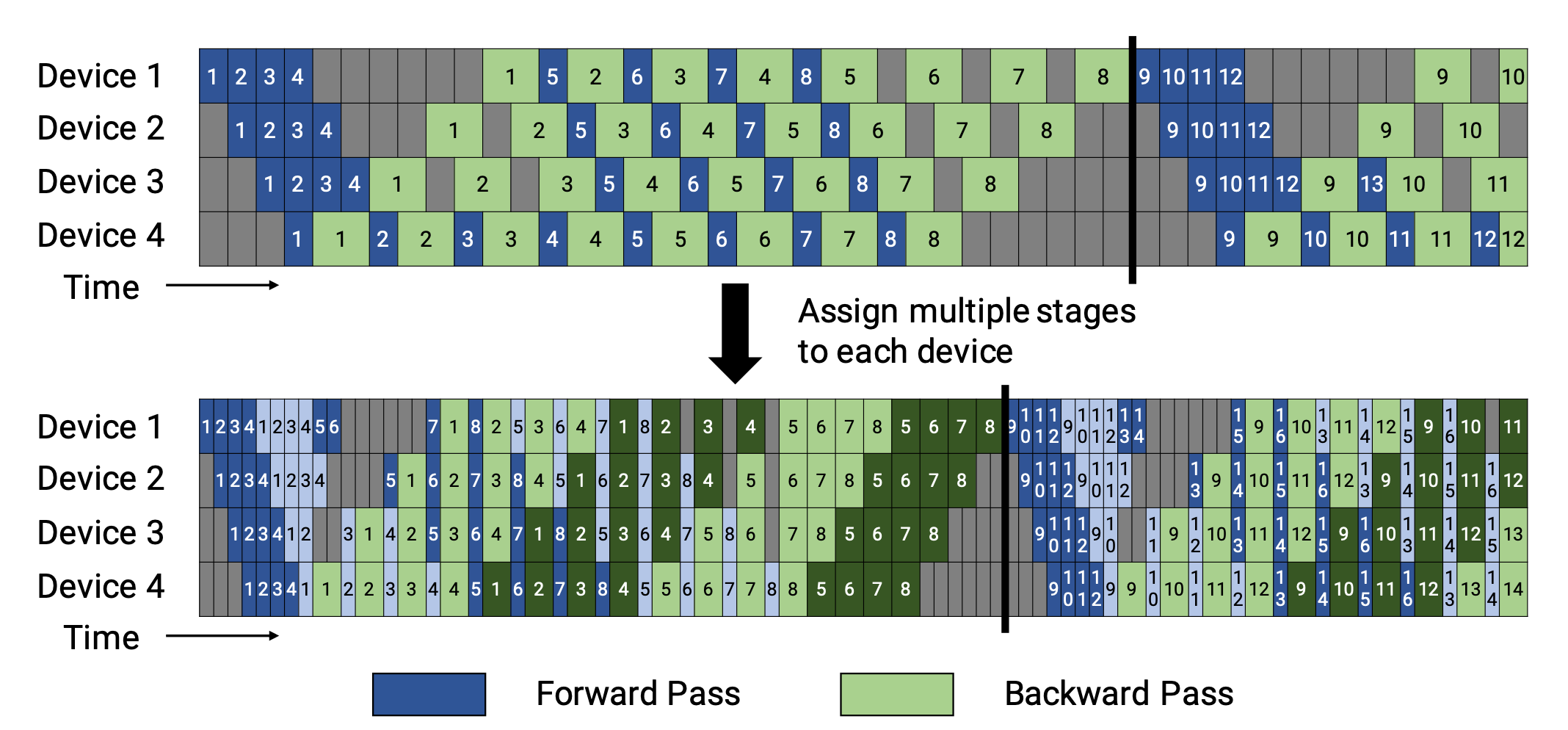
Narayanan et al. (2021) combine pipeline, tensor, and data parallelism with a new pipeline scheduling strategy, calling the approach PTD-P. Rather than assigning a single continuous set of layers (a “model chunk”) to each device, each worker can receive multiple chunks, each chunk being a smaller continuous subset of layers (for example, device 1 holds layers 1, 2, 9, 10; device 2 holds layers 3, 4, 11, 12; each has two model chunks). The number of microbatches per batch must be exactly divisible by the number of workers ($m % d = 0$). If there are $v$ model chunks per worker, then pipeline bubble time can be reduced by a factor of $v$ relative to GPipe scheduling.

Mixture-of-Experts (MoE)

The Mixture-of-Experts (MoE) approach has attracted substantial recent attention as researchers (primarily at Google) push the limits of model size. The central idea is borrowed from ensembling learning: combining multiple weak learners can yield a strong learner.

Within a single deep neural network, ensembling can be implemented via a gating mechanism that connects multiple experts (Shazeer et al., 2017). The gating mechanism decides which subset of the network (for example, which experts) should be activated to produce outputs. The paper refers to this as a “sparsely gated mixture-of-experts” (MoE) layer.

More specifically, one MoE layer contains:

• $n$ feed-forward networks as experts $\{E_i\}^n_{i=1}$
• A trainable gating network $G$ that learns a probability distribution over $n$ experts in order to route traffic to a small set of selected experts.

Because the gating outputs determine which experts are evaluated, not every expert must be computed for every input. When the number of experts becomes very large, a two-level hierarchical MoE can be considered.

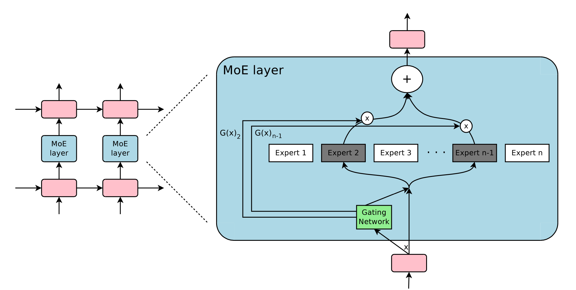
A basic choice for $G$ is to multiply the input by a trainable weight matrix $G_g$ and then apply softmax: $G_\sigma (x) = \text{softmax}(x W_g)$. However, this produces a dense gating control vector and does not reduce computation, since an expert is unnecessary to evaluate only when $G^{(i)}(x)=0$. Therefore, the MoE layer retains only the top $k$ values. It also injects tunable Gaussian noise into $G$ to improve load balancing. This is known as noisy top-k gating.

Here, the superscript $v^{(i)}$ denotes the i-th dimension of the vector $v$. The function $\text{topk}(., k)$ selects the top $k$ dimensions with the largest values by setting all other dimensions to $-\infty$.

To counteract a self-reinforcing dynamic in which the gating network repeatedly prefers a small set of strong experts, Shazeer et al. (2017) introduce a soft constraint implemented as an additional importance loss that encourages experts to receive similar weights. This loss is equivalent to the squared coefficient of variation of the batchwise average value per expert.

where $ \text{CV}$ is the coefficient of variation, and the loss weight $w_\text{aux}$ is a tunable hyperparameter.

Because each expert network receives only a fraction of the training examples (the “shrinking batch problem”), MoE generally benefits from using as large a batch size as possible. However, batch size is constrained by GPU memory, so data parallelism and model parallelism are often applied to increase throughput.

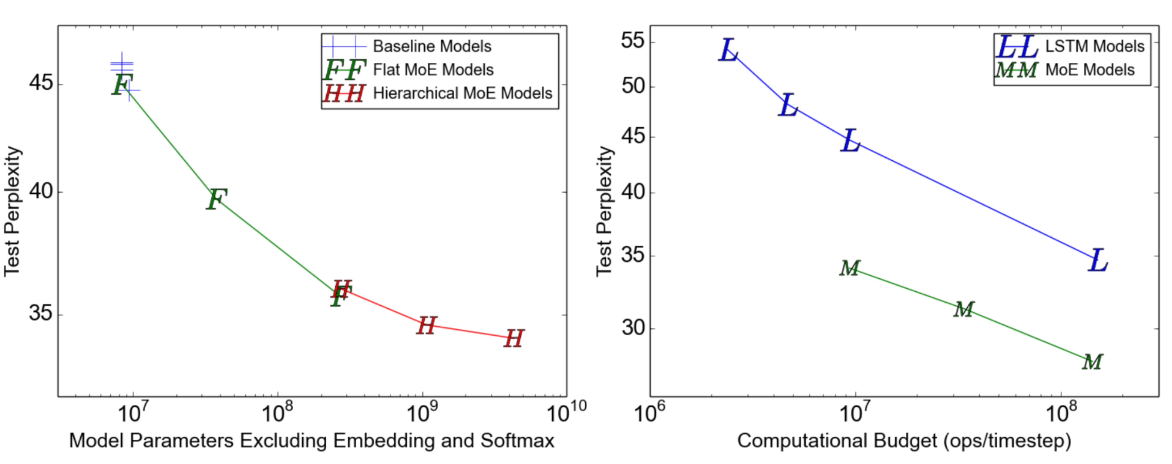
GShard (Lepikhin et al., 2020) scales MoE transformer models to 600 billion parameters using sharding. In the MoE transformer, every other feed-forward layer is replaced with an MoE layer. The sharded MoE transformer shards only the MoE layers across machines, while duplicating the remaining layers.

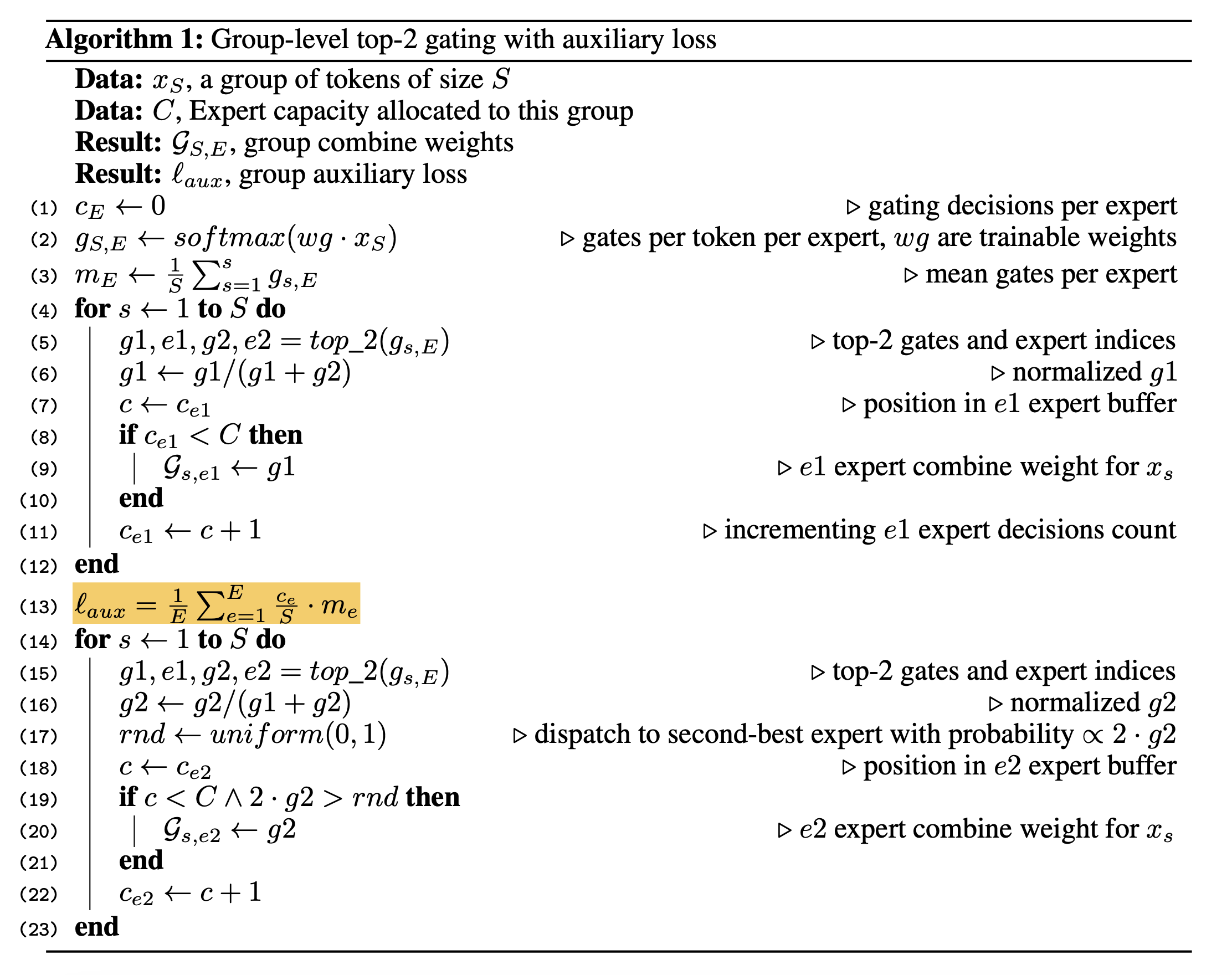
GShard introduces several refinements to the gating function $G$:

• Expert capacity: The number of tokens processed by an expert must not exceed a threshold called “expert capacity.” If a token is routed to experts that have already reached capacity, that token is marked as “overflowed,” and the gating output is set to a zero vector.
• Local group dispatching: Tokens are evenly split into multiple local groups, and expert capacity is enforced at the group level.
• Auxiliary loss: Motivated similarly to the original MoE auxiliary loss, an auxiliary term is added to minimize the mean square of the fraction of data routed to each expert.
• Random routing: The second-best expert is chosen with probability proportional to its weight; otherwise, GShard uses random routing to introduce additional randomness.

Switch Transformer (Fedus et al. 2021) scales model size to trillions of parameters (!!) by replacing the dense feed-forward layer with a sparse switch FFN layer, where each input is routed to exactly one expert network. The load-balancing auxiliary loss is $\text{loss}_\text{aux} = w_\text{aux} \sum_{i=1}^n f_i p_i$ for $n$ experts, where $f_i$ is the fraction of tokens routed to the $i$-th expert and $p_i$ is the routing probability for expert $i$ predicted by the gating network.

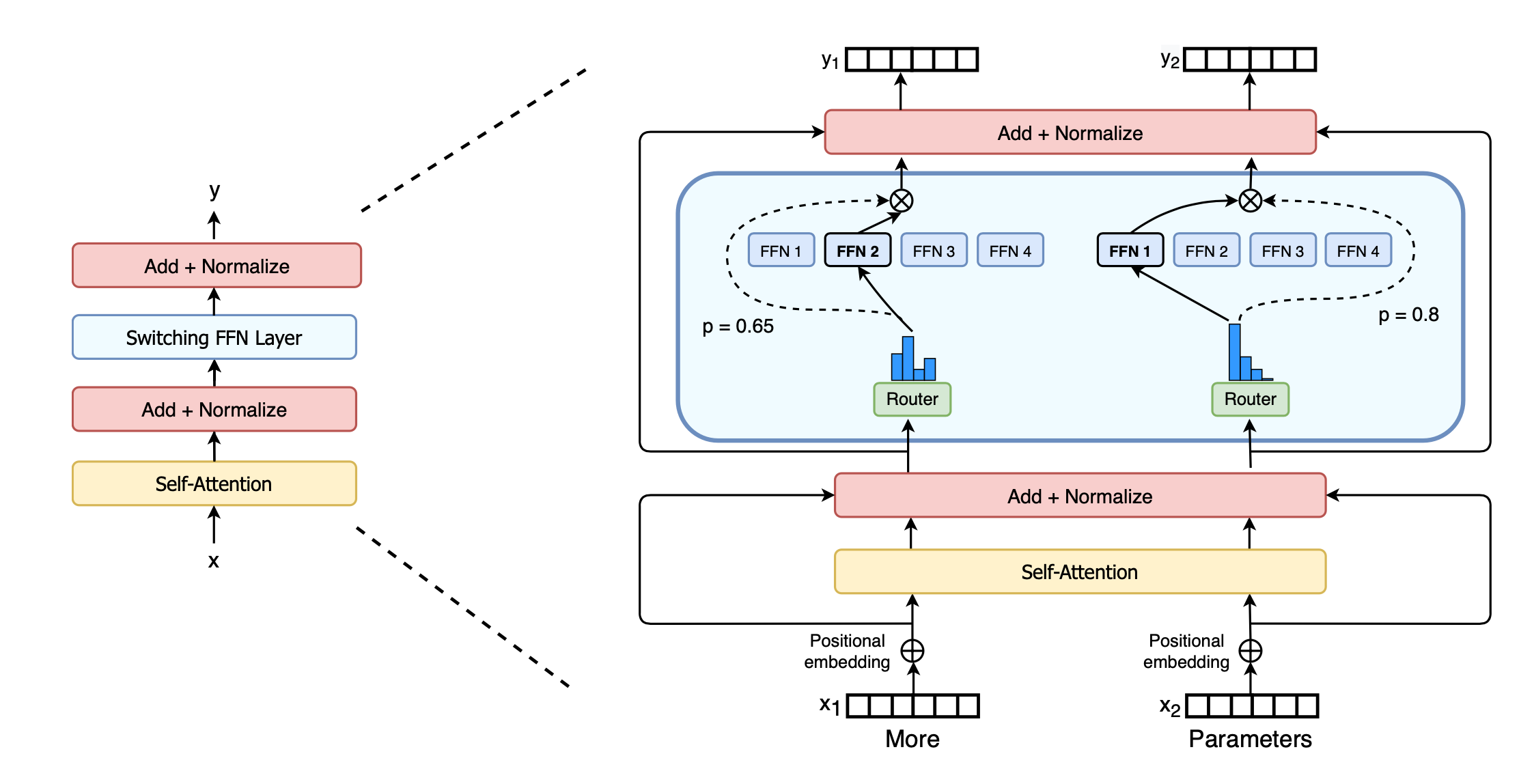
To improve training stability, Switch Transformer incorporates the following techniques:

• Selective precision: The authors show that selectively casting only a local portion of the model to FP32 improves stability while avoiding the high communication overhead of FP32 tensors. FP32 is applied only within the body of the router function, after which results are cast back to FP16.
• Smaller initialization: Weight matrices are initialized from a truncated normal distribution with mean $\mu=0$ and stdev $\sigma = \sqrt{s/n}$. They also recommend reducing the transformer initialization scale parameter from $s=1$ to $s=0.1$.
• Use higher expert dropout: Fine-tuning often uses small datasets; to reduce overfitting, the dropout rate within each expert is increased substantially. The paper notes that increasing dropout across all layers hurts performance. In their setup, dropout is 0.1 for non-expert layers and 0.4 within expert FF layers.

The Switch Transformer paper also provides a helpful illustration summarizing data and model parallelism strategies for training large models:

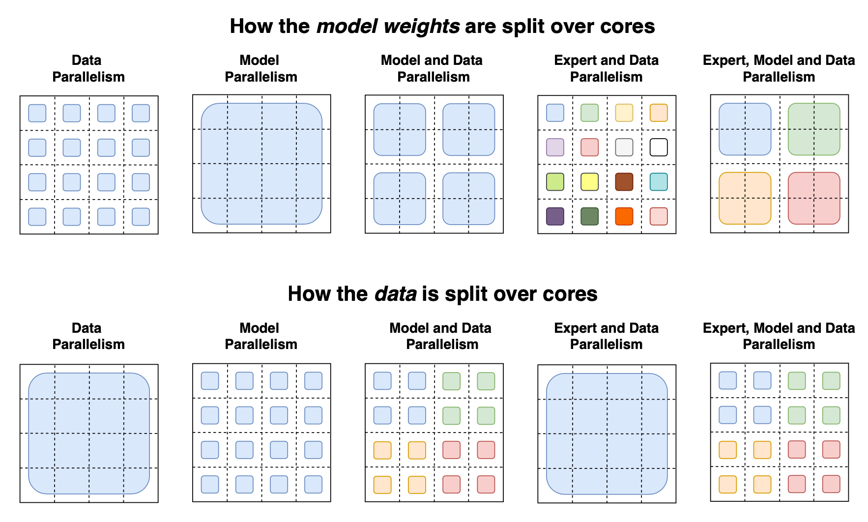
Both GShard top-2 and Switch Transformer top-1 rely on token choice, where each token selects the best one or two experts for routing. Both use an auxiliary loss to encourage more balanced load allocation, but this does not guarantee optimal performance. In addition, the expert capacity limit can waste tokens, since tokens may be dropped if an expert reaches capacity.

Export Choice (EC) (Zhou et al. 2022) routing instead allows each expert to select the top-$k$ tokens. This means each expert naturally enforces a fixed capacity, and a token can be routed to multiple experts. EC achieves perfect load balancing and is reported to improve training convergence by 2x.

With $e$ experts and an input matrix $X \in \mathbb{R}^{n \times d}$, the token-to-expert affinity scores are computed as: $ S = \text{softmax}(X \cdot W_g), \text{where } W_g \in \mathbb{R}^{d \times e}, S \in \mathbb{R}^{n \times e} $

A token-to-expert assignment is represented by three matrices, $I, G \in \mathbb{R}^{e\times k}$ and $P \in \mathbb{R}^{e \times k \times n}$. $I[i,j]$ indicates which token is the $j$-th selection made by the $i$-th expert. The gating matrix $G$ stores routing weights for the selected tokens. $P$ is the one-hot form of $I$, and it is used to produce the input matrix ($P \cdot X \in \mathbb{R}^{e \times k \times d}$) for the gated FFN layer. $ G, I = \text{top-k}(S^\top, k)\quad P = \text{one-hot}(I) $

One regularization explored for expert choice routing is to limit the maximum number of experts per token.

where each entry $A[i,j]$ in $A \in \mathbb{R}^{e \times n}$ indicates whether the $i$-th expert selects the $j$-th token. Solving this is non-trivial. The paper uses Dykstra’s algorithm, which runs a sequence of multiple iterative computation steps. In the experiments, capped expert choice leads to a slight decrease in fine-tuning performance.

The parameter $k$ is set by $k=nc/e$, where $n$ is the total number of tokens in a batch and $c$ is a capacity factor representing the average number of experts used per token. The paper uses $c=2$ in most experiments, but EC with $c=1$ still outperforms top-1 token choice gating. Interestingly, $c=0.5$ only slightly harms training performance.

A major limitation of EC is that it does not work when batch size is too small, and it also does not apply to auto-regressive text generation, because it must know future tokens to perform the top-$k$ selection.

Other Memory Saving Designs

CPU Offloading

When GPU memory is exhausted, one option is to offload temporarily unused data to the CPU and load it back later when needed (Rhu et al. 2016). The concept of CPU offloading is straightforward, but it has become less common in recent years due to the training-time slowdown it introduces.

Activation Recomputation

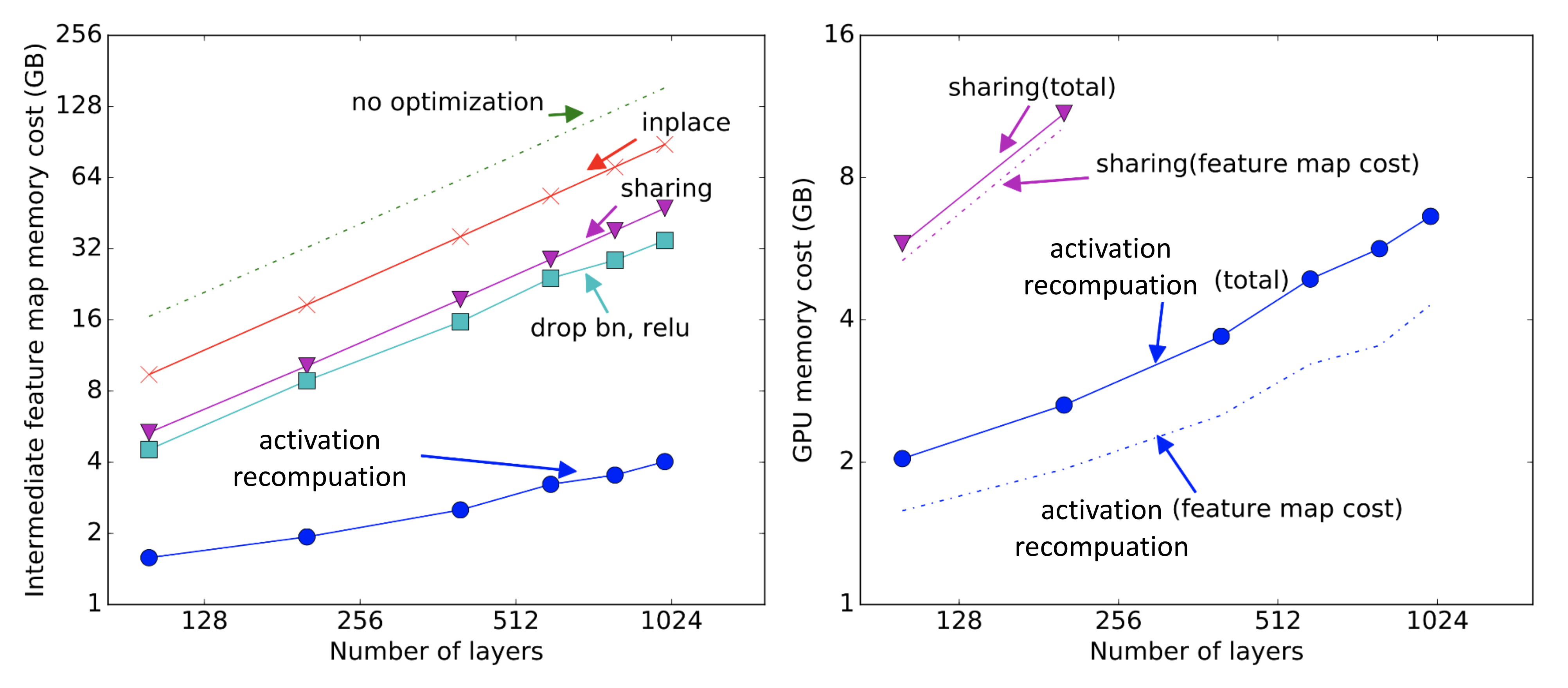
Activation recomputation (also referred to as “activation checkpointing” or “gradient checkpointing”; Chen et al. 2016) is a straightforward but effective technique for reducing the memory footprint, trading memory savings for additional computation. It lowers the memory required to train a $\ell$-layer deep neural network to $O(\sqrt{\ell})$, at the cost of one additional forward-pass computation per batch.

Assume we evenly split an $\ell$-layer network into $d$ partitions. Only the activations at partition boundaries are stored and communicated across workers. Activations within each partition are still required for gradient computation, so they are recomputed during the backward pass. Under activation recomputation, the memory cost for training $M(\ell)$ is:

The minimum memory cost is $O(\sqrt{\ell})$ when $d=\sqrt{\ell}$.

This activation recomputation technique can achieve sublinear memory growth with respect to model size.

Mixed Precision Training

Narang & Micikevicius et al. (2018) proposed an approach for training models with half-precision floating point (FP16) values without sacrificing model accuracy.

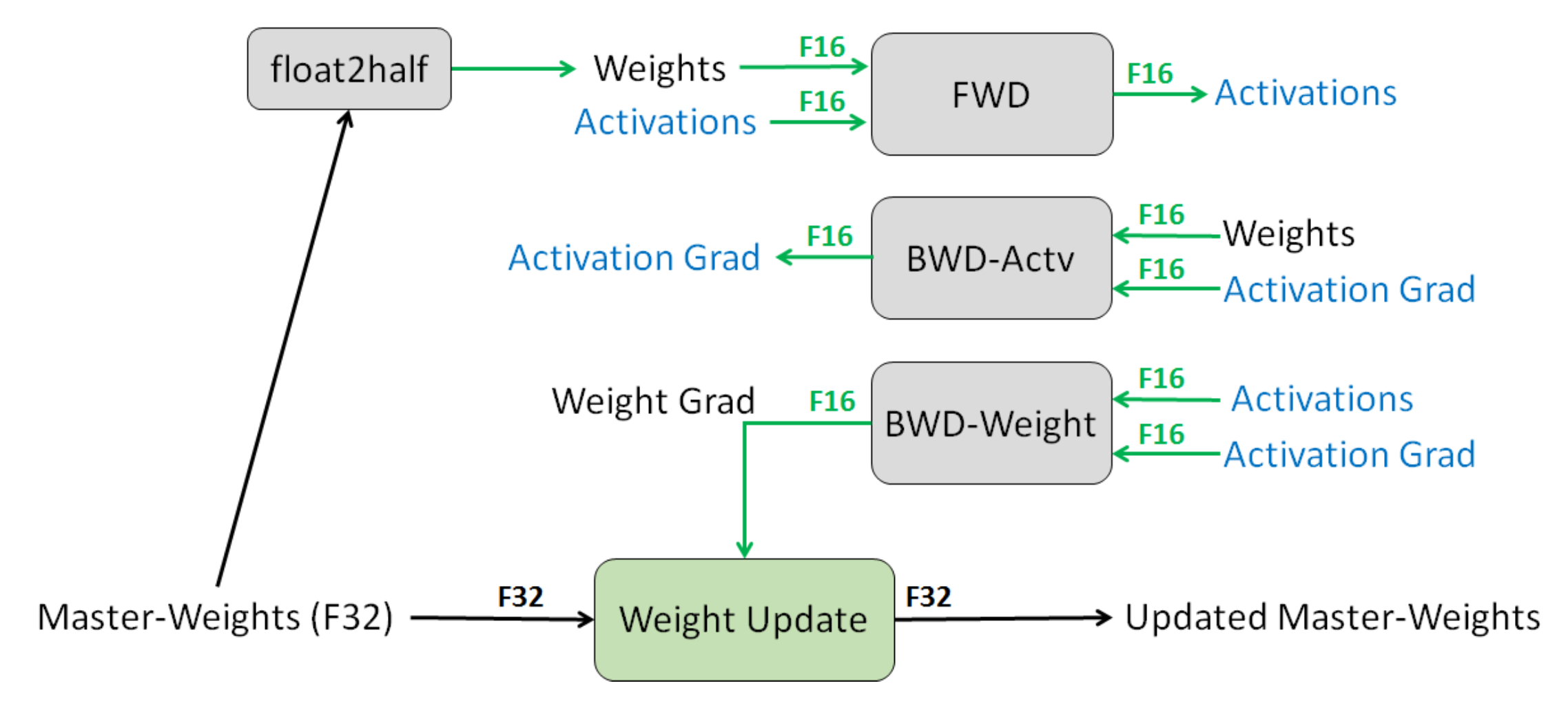
They highlight three techniques for preventing the loss of important information when using half-precision:

• Full-precision master copy of weights. Keep an FP32 copy of the model weights to accumulate gradients. For the forward and backward passes, values are rounded to half precision. This is motivated by the fact that each gradient update (that is, gradient multiplied by the learning rate) can be too small to be represented within the FP16 range (that is, $2^{-24}$ becomes zero in FP16).
• Loss scaling. Multiply the loss by a scaling factor to better accommodate small-magnitude gradients (see Fig. 16). Scaling increases gradient magnitudes so that more values shift into the larger, representable region of the range, preserving values that would otherwise underflow.
• Arithmetic precision. For common network computations (for example, vector dot products and reductions that sum vector elements), partial sums can be accumulated in FP32, then the final output is stored as FP16 before being written to memory. Point-wise operations may be executed in either FP16 or FP32.

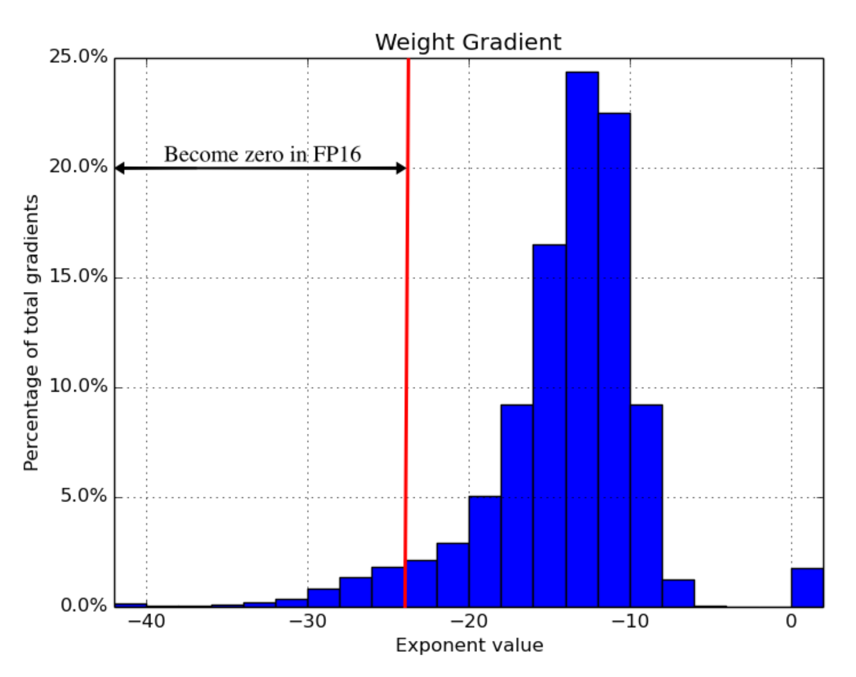
In their experiments, loss scaling was unnecessary for certain networks (for example, image classification and Faster R-CNN) but required for others (for example, Multibox SSD and a large LSTM language model).

Compression

Intermediate results often dominate memory usage, even though they are only needed once during the forward pass and once during the backward pass. Because there is a clear temporal gap between these two uses, Jain et al. (2018) proposed a data-encoding strategy that compresses intermediate results after their first use in the forward pass, then decompresses them later for backpropagation.

Their system, Gist, includes two encoding schemes: Layer-specific lossless encoding, which targets ReLU-Pool (“Binarize”) and ReLU-Conv (“Sparse storage and dense computation”) patterns. Aggressive lossy encoding, which applies delayed precision reduction (DPR). They observed that feature maps should be preserved at high precision for their first immediate use, while the second use can tolerate reduced precision.

Experimental results showed that Gist reduces memory cost by 2x across five SOTA image-classification DNNs, averaging 1.8x reduction with only 4% performance overhead.

Memory Efficient Optimizer

Optimizers can be especially memory-intensive. For example, the widely used Adam optimizer must maintain momentums and variances, each comparable in size to the gradients and model parameters. As a result, training can suddenly require 4x the memory of the model weights alone.

Multiple optimizers have been introduced to lower this memory footprint. For instance, rather than storing full momentums and variances as Adam does, Adafactor (Shazeer et al. 2018) tracks only per-row and per-column sums of moving averages, then estimates second moments from these sums. SM3 (Anil et al. 2019) presents a different adaptive optimization method that also substantially reduces memory usage.

ZeRO (Zero Redundancy Optimizer; Rajbhandari et al. 2019) reduces training memory for large models based on observations about the two primary sources of memory consumption during large-model training:

1. Most memory is taken by model states, including optimizer states (for example, Adam momentums and variances), gradients, and parameters. Mixed-precision training increases memory demands because the optimizer must maintain an FP32 copy of parameters and other optimizer states in addition to the FP16 version.
2. The remainder is used by activations, temporary buffers, and unusable fragmented memory (referred to as residual states in the paper).

ZeRO integrates two approaches, ZeRO-DP and ZeRO-R. ZeRO-DP extends data parallelism to eliminate straightforward redundancy in model states. It partitions optimizer state, gradients, and parameters across multiple data-parallel processes using a dynamic communication schedule to minimize communication volume. ZeRO-R reduces memory usage associated with residual states through partitioned activation recomputation, constant buffer sizing, and on-the-fly memory defragmentation.

Citation

Cited as:

Weng, Lilian. (Sep 2021). How to train really large models on many GPUs? Lil’Log. https://lilianweng.github.io/posts/2021-09-25-train-large/.

Or

@article{weng2021large,
  title   = "How to Train Really Large Models on Many GPUs?",
  author  = "Weng, Lilian",
  journal = "lilianweng.github.io",
  year    = "2021",
  month   = "Sep",
  url     = "https://lilianweng.github.io/posts/2021-09-25-train-large/"
}

References

[1] Li et al. “PyTorch Distributed: Experiences on Accelerating Data Parallel Training” VLDB 2020.

[2] Cui et al. “GeePS: Scalable deep learning on distributed GPUs with a GPU-specialized parameter server” EuroSys 2016

[3] Shoeybi et al. “Megatron-LM: Training Multi-Billion Parameter Language Models Using Model Parallelism.” arXiv preprint arXiv:1909.08053 (2019).

[4] Narayanan et al. “Efficient Large-Scale Language Model Training on GPU Clusters Using Megatron-LM.” arXiv preprint arXiv:2104.04473 (2021).

[5] Huang et al. “GPipe: Efficient Training of Giant Neural Networks using Pipeline Parallelism.” arXiv preprint arXiv:1811.06965 (2018).

[6] Narayanan et al. “PipeDream: Generalized Pipeline Parallelism for DNN Training.” SOSP 2019.

[7] Narayanan et al. “Memory-Efficient Pipeline-Parallel DNN Training.” ICML 2021.

[8] Shazeer et al. “The Sparsely-Gated Mixture-of-Experts Layer Noam.” arXiv preprint arXiv:1701.06538 (2017).

[9] Lepikhin et al. “GShard: Scaling Giant Models with Conditional Computation and Automatic Sharding.” arXiv preprint arXiv:2006.16668 (2020).

[10] Fedus et al. “Switch Transformers: Scaling to Trillion Parameter Models with Simple and Efficient Sparsity.” arXiv preprint arXiv:2101.03961 (2021).

[11] Narang & Micikevicius, et al. “Mixed precision training.” ICLR 2018.

[12] Chen et al. 2016 “Training Deep Nets with Sublinear Memory Cost.” arXiv preprint arXiv:1604.06174 (2016).

[13] Jain et al. “Gist: Efficient data encoding for deep neural network training.” ISCA 2018.

[14] Shazeer & Stern. “Adafactor: Adaptive learning rates with sublinear memory cost.” arXiv preprint arXiv:1804.04235 (2018).

[15] Anil et al. “Memory-Efficient Adaptive Optimization.” arXiv preprint arXiv:1901.11150 (2019).

[16] Rajbhandari et al. “ZeRO: Memory Optimization Towards Training A Trillion Parameter Models Samyam.” arXiv preprint arXiv:1910.02054 (2019).

[17] Zhou et al. “Mixture-of-Experts with Expert Choice Routing” arXiv preprint arXiv:2202.09368 (2022).