Learning with Insufficient Data, Part 1: Semi-Supervised Learning
When supervised learning tasks must be addressed with only a small amount of labeled data, four commonly cited approaches are typically considered.
· 26 min read · Curated and presented by Arthur Sedek
When supervised learning must be done with only a limited quantity of labeled data, four approaches are commonly considered.
- Pre-training + fine-tuning: Pre-train a strong, task-agnostic model on a large unsupervised corpus, for example, pre-training LMs on free text, or pre-training vision models on unlabeled images via self-supervised learning; then fine-tune the model on the downstream task using a small set of labeled examples.
- Semi-supervised learning: Train jointly on labeled and unlabeled samples. This approach has been studied extensively in vision.
- Active learning: Labeling is expensive, yet additional labels may still be desirable under a fixed budget. Active learning aims to select the most valuable unlabeled samples to label next, enabling more effective use of limited labeling resources.
- Pre-training + dataset auto-generation: With a capable pre-trained model, it becomes possible to automatically generate many additional labeled samples. This direction has been particularly popular in language, motivated by the success of few-shot learning.
I plan to write a series of posts on the topic of “Learning with not enough data”. Part 1 focuses on Semi-Supervised Learning.
What is semi-supervised learning?
Semi-supervised learning trains a model using both labeled and unlabeled data.
Notably, much of the existing semi-supervised learning literature concentrates on vision tasks. In contrast, for language tasks, pre-training plus fine-tuning is a more common paradigm.
All methods introduced in this post use a loss that combines two components: $\mathcal{L} = \mathcal{L}_s + \mu(t) \mathcal{L}_u$. The supervised loss $\mathcal{L}_s$ is straightforward to compute from the labeled examples. Here, we concentrate on how the unsupervised loss $\mathcal{L}_u$ is constructed. A typical choice for the weighting term $\mu(t)$ is a ramp function that increases the importance of $\mathcal{L}_u$ over time, where $t$ denotes the training step.
Disclaimer: This post does not cover semi-supervised methods that primarily modify model architecture. For approaches using generative models and graph-based methods in semi-supervised learning, see this survey.
Notations
| Symbol | Meaning |
|---|---|
| $L$ | Number of unique labels. |
| $(\mathbf{x}^l, y) \sim \mathcal{X}, y \in \{0, 1\}^L$ | Labeled dataset. $y$ is a one-hot representation of the true label. |
| $\mathbf{u} \sim \mathcal{U}$ | Unlabeled dataset. |
| $\mathcal{D} = \mathcal{X} \cup \mathcal{U}$ | The entire dataset, including both labeled and unlabeled examples. |
| $\mathbf{x}$ | Any sample which can be either labeled or unlabeled. |
| $\bar{\mathbf{x}}$ | $\mathbf{x}$ with augmentation applied. |
| $\mathbf{x}_i$ | The $i$-th sample. |
| $\mathcal{L}$, $\mathcal{L}_s$, $\mathcal{L}_u$ | Loss, supervised loss, and unsupervised loss. |
| $\mu(t)$ | The unsupervised loss weight, increasing in time. |
| $p(y \vert \mathbf{x}), p_\theta(y \vert \mathbf{x})$ | The conditional probability over the label set given the input. |
| $f_\theta(.)$ | The implemented neural network with weights $\theta$, the model that we want to train. |
| $\mathbf{z} = f_\theta(\mathbf{x})$ | A vector of logits output by $f$. |
| $\hat{y} = \text{softmax}(\mathbf{z})$ | The predicted label distribution. |
| $D[.,.]$ | A distance function between two distributions, such as MSE, cross entropy, KL divergence, etc. |
| $\beta$ | EMA weighting hyperparameter for teacher model weights. |
| $\alpha, \lambda$ | Parameters for MixUp, $\lambda \sim \text{Beta}(\alpha, \alpha)$. |
| $T$ | Temperature for sharpening the predicted distribution. |
| $\tau$ | A confidence threshold for selecting the qualified prediction. |
Hypotheses
Several hypotheses in the literature are commonly used to justify key design choices in semi-supervised learning methods.
-
H1: Smoothness Assumptions: If two data samples are close to each other in a high-density region of the feature space, their labels should be identical or very similar.
-
H2: Cluster Assumptions: The feature space contains both dense and sparse regions. Data points that are densely grouped naturally form clusters, and samples within the same cluster are expected to share the same label. This can be viewed as a modest extension of H1.
-
H3: Low-density Separation Assumptions: Decision boundaries between classes tend to lie in sparse, low-density regions. Otherwise, a boundary would cut through a high-density cluster and split it into two classes, effectively creating two clusters and violating H1 and H2.
-
H4: Manifold Assumptions: High-dimensional data often lie on a low-dimensional manifold. Although real-world data may be observed in very high dimensions (for example, images of real-world objects or scenes), such data can often be represented by a lower-dimensional manifold that captures key attributes and places similar points close together (for example, images of real-world objects or scenes are not drawn from a uniform distribution over all pixel combinations). This assumption supports learning more efficient representations that make it easier to discover and quantify similarity between unlabeled points. It is also a foundation for representation learning. [see a helpful link].
Consistency Regularization
Consistency Regularization (also called Consistency Training) is based on the assumption that randomness in the neural network (for example, Dropout) or data-augmentation transformations should not change the model’s prediction for the same underlying input. Every method in this section includes a consistency regularization loss of the form $\mathcal{L}_u$.
This idea also appears in several self-supervised learning methods, such as SimCLR, BYOL, SimCSE, and others, where different augmented views of the same sample are expected to yield the same representation. Related motivations are shared by Cross-view training in language modeling and multi-view learning in self-supervised learning.
Π-model

Sajjadi et al. (2016) proposed an unsupervised loss that minimizes the discrepancy between two passes through the same network, using stochastic transformations (for example, dropout or random max-pooling) applied to the same data point. Because the label is not used explicitly, the loss can be applied to unlabeled data. Laine & Aila (2017) later introduced the term Π-Model for this configuration.
where $f’$ denotes the same neural network evaluated with different stochastic augmentation or dropout masks. This loss is computed over the entire dataset.
Temporal ensembling
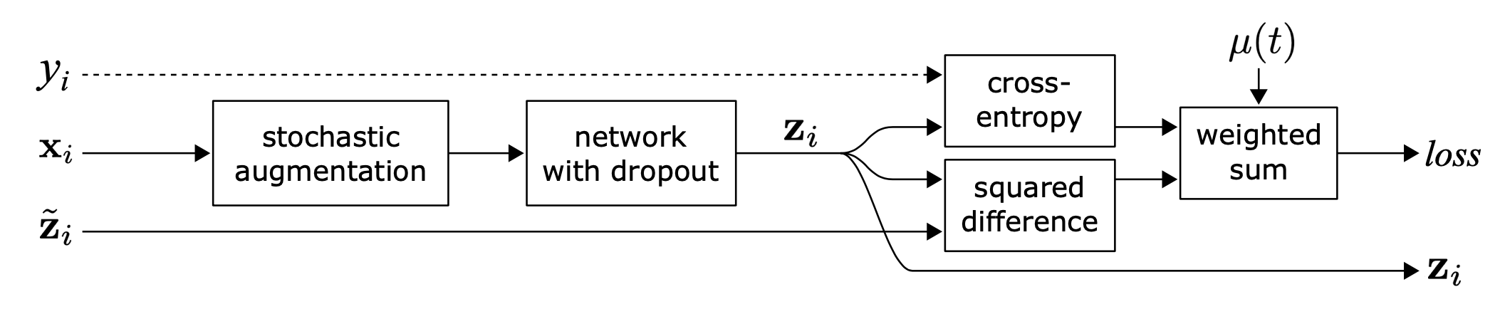
The Π-model requires two forward passes per sample, effectively doubling compute. To reduce this overhead, Temporal Ensembling (Laine & Aila 2017) maintains an exponential moving average (EMA) of the model’s prediction over time for each training sample $\tilde{\mathbf{z}}_i$, and uses that EMA as the learning target. This target is evaluated and updated only once per epoch. Because the ensemble output $\tilde{\mathbf{z}}_i$ is initialized to $\mathbf{0}$, it is normalized by $(1-\alpha^t)$ to correct startup bias. The Adam optimizer uses similar bias correction terms for the same reason.
where $\tilde{\mathbf{z}}^{(t)}$ is the ensemble prediction at epoch $t$, and $\mathbf{z}_i$ is the model prediction in the current round. Note that since $\tilde{\mathbf{z}}^{(0)} = \mathbf{0}$, with correction, $\tilde{\mathbf{z}}^{(1)}$ is simply equivalent to $\mathbf{z}_i$ at epoch 1.
Mean teachers
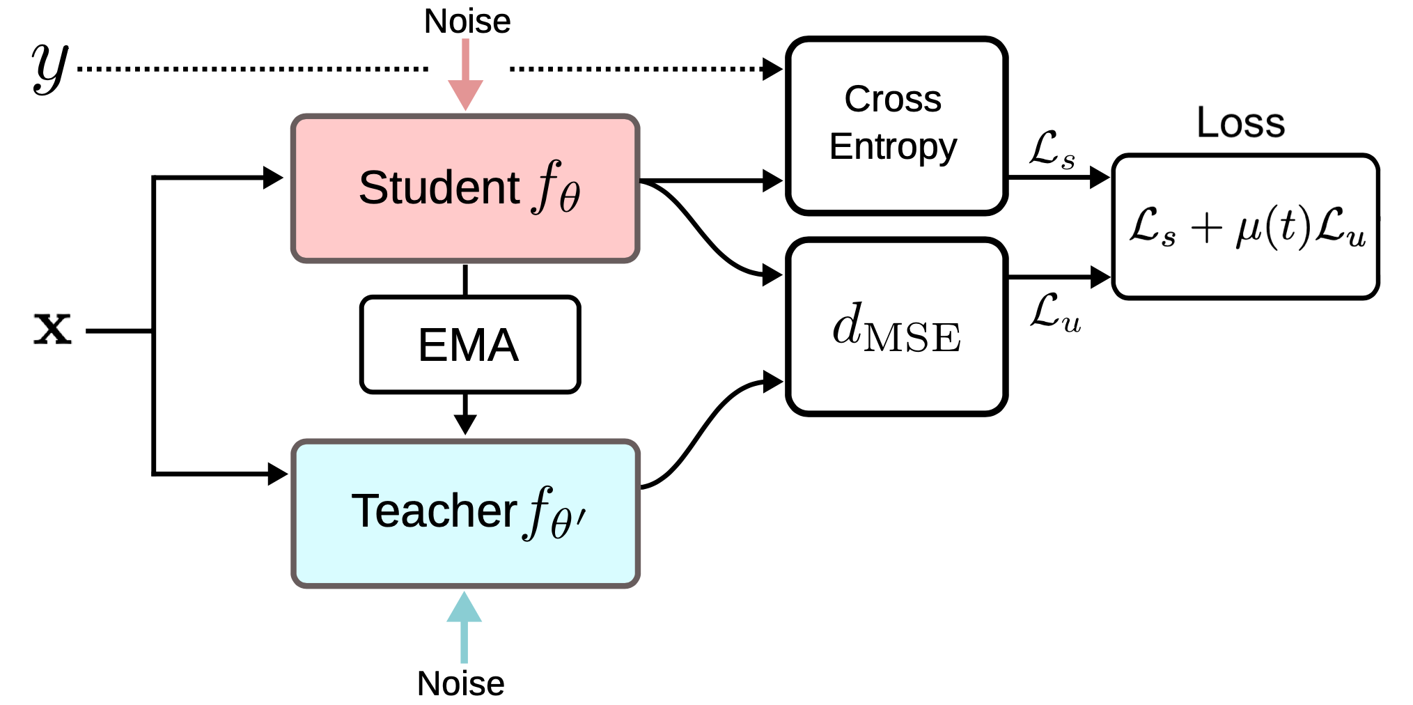
Temporal Ensembling stores an EMA of label predictions per training sample as the learning target. However, because this prediction changes only once per epoch, the target update becomes awkward for large datasets. Mean Teacher (Tarvaninen & Valpola, 2017) addresses this slow update by tracking an EMA of model weights rather than model outputs. Denote the original model with weights $\theta$ as the student model, and the model with moving-averaged weights $\theta’$ across consecutive student models as the mean teacher: $\theta’ \gets \beta \theta’ + (1-\beta)\theta$
The consistency regularization loss is defined as the distance between the student’s and teacher’s predictions, and the student-teacher discrepancy is minimized. The mean teacher is expected to generate more accurate predictions than the student. This is confirmed empirically, as shown in
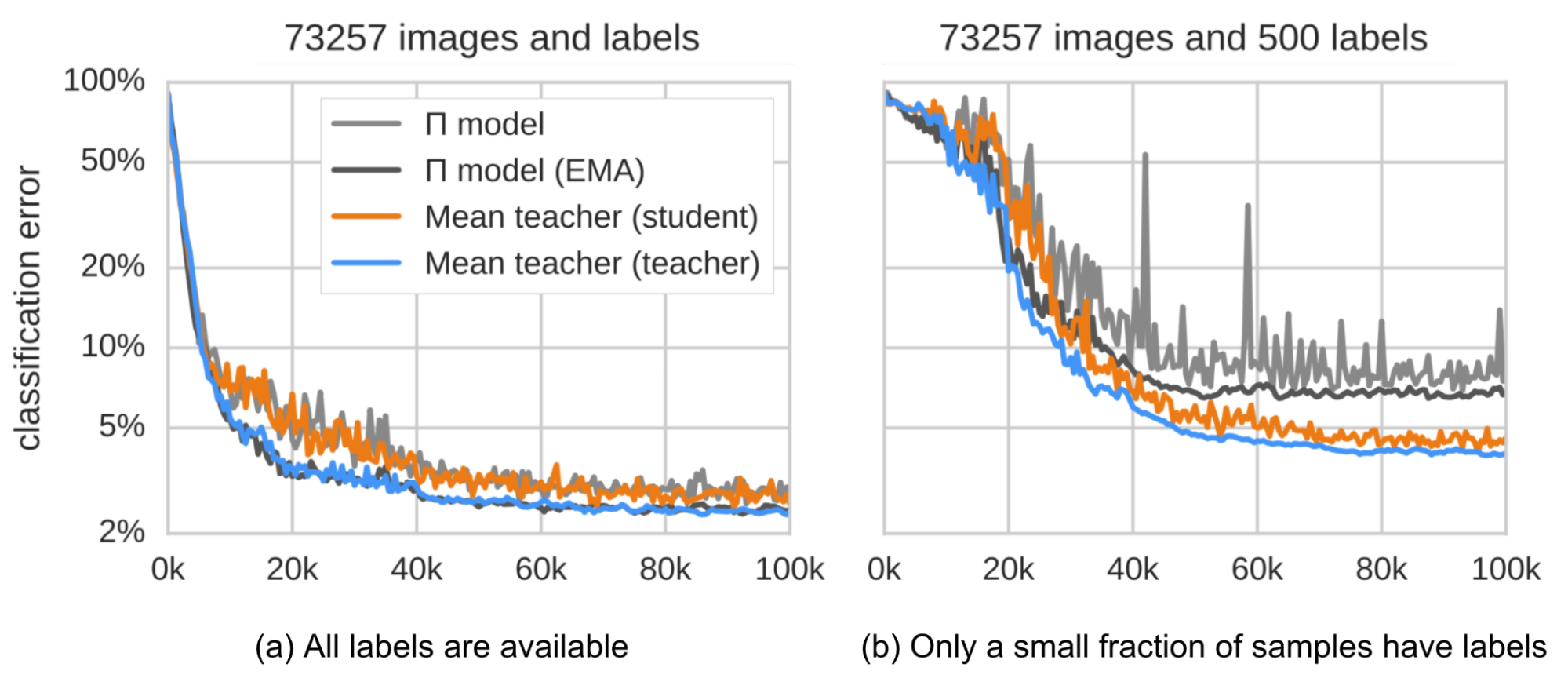
Based on their ablation studies:
- Input augmentation (for example, random flips of input images and Gaussian noise) or student-model dropout is necessary for strong performance. Dropout is not needed in the teacher model.
- Performance is sensitive to the EMA decay hyperparameter $\beta$. A practical strategy is to use a smaller $\beta=0.99$ during the ramp-up stage, and a larger $\beta=0.999$ later, when student improvements slow down.
- They report that MSE as the consistency cost performs better than alternative cost functions such as KL divergence.
Noisy samples as learning targets
Several more recent consistency training methods minimize prediction differences between an original unlabeled sample and an augmented version of that sample. This resembles the Π-model, but the consistency regularization loss is applied only to unlabeled data.
Adversarial Training (Goodfellow et al. 2014) adds adversarial perturbations to the input and trains the model to be robust to such attacks. In supervised learning, the setup is:
where $q(y \mid \mathbf{x}^l)$ is the true distribution, approximated by one-hot encoding of the ground truth label, $y$. $p_\theta(y \mid \mathbf{x}^l)$ is the model prediction. $D[.,.]$ is a distance function that measures divergence between two distributions.
Virtual Adversarial Training (VAT; Miyato et al. 2018) extends this idea to semi-supervised learning. Since $q(y \mid \mathbf{x}^l)$ is unknown, VAT replaces it with the current model prediction for the original input under the current weights $\hat{\theta}$. Note that $\hat{\theta}$ is a fixed copy of the model weights, so there is no gradient update on $\hat{\theta}$.
The VAT loss is applied to both labeled and unlabeled samples. It serves as a negative smoothness measure of the current model’s prediction manifold at each data point, and optimizing it encourages the manifold to become smoother.
Interpolation Consistency Training (ICT; Verma et al. 2019) augments the dataset by adding interpolations of data points and encourages the model to be consistent with interpolations of the corresponding labels. The MixUp (Zheng et al. 2018) operation mixes two images via a simple weighted sum and combines it with label smoothing. Following MixUp, ICT trains the model so that the prediction on a mixup sample matches the interpolation of the predictions on the corresponding inputs:
where $\theta’$ is a moving average of $\theta$, which is a mean teacher.
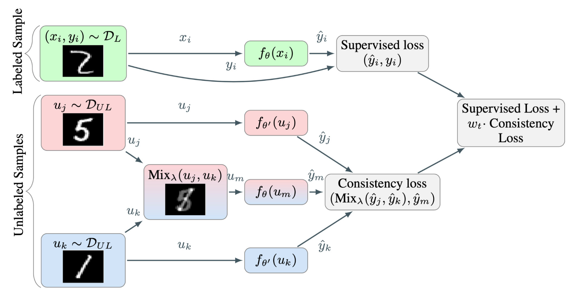
Because two randomly selected unlabeled samples are likely to come from different classes (for example, ImageNet contains 1000 object classes), applying mixup between two random unlabeled samples is likely to produce interpolations near a decision boundary. Under the low-density separation assumptions, decision boundaries tend to lie in low-density regions.
where $\theta’$ is a moving average of $\theta$.
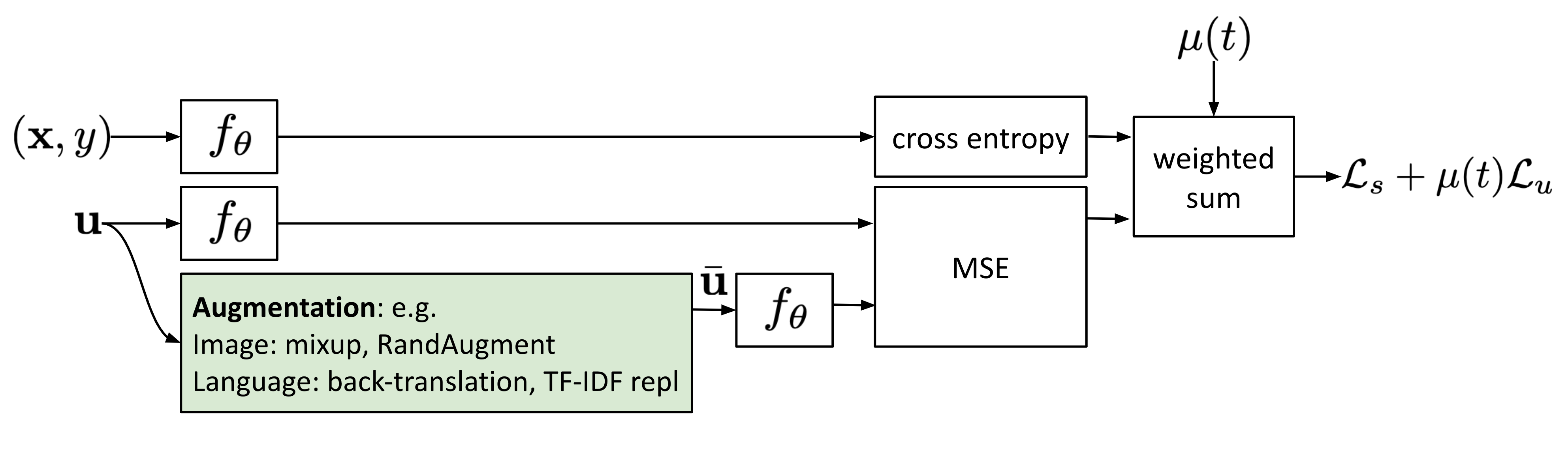
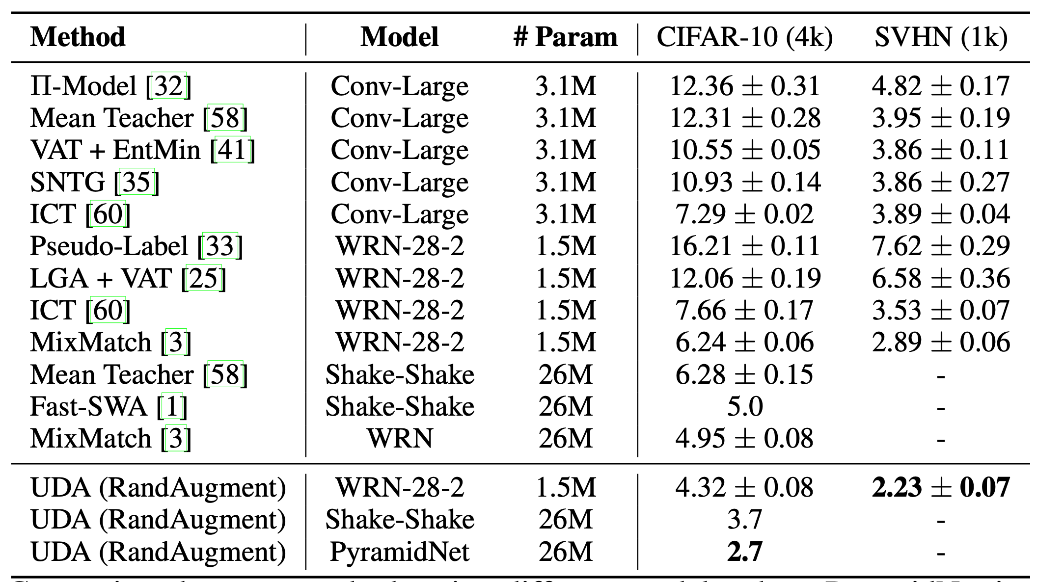
Similar to VAT, Unsupervised Data Augmentation (UDA; Xie et al. 2020) trains the model to produce the same output for an unlabeled example and its augmented counterpart. UDA specifically investigates how the “quality” of noise influences semi-supervised performance under consistency training. Using strong data augmentation is crucial for generating meaningful and effective noisy samples. Effective augmentation should produce noise that is valid (that is, it does not change the label) and diverse, and it should introduce targeted inductive biases.
For images, UDA uses RandAugment (Cubuk et al. 2019), which uniformly samples augmentation operations available in PIL. It requires no learning or optimization and is therefore much cheaper than AutoAugment.
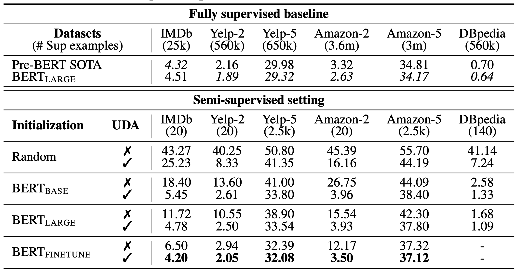
For language, UDA combines back-translation with TF-IDF-based word replacement. Back-translation preserves high-level meaning but may not keep specific words, while TF-IDF-based replacement drops uninformative words with low TF-IDF scores. In experiments on language tasks, they found UDA to be complementary to transfer learning and representation learning; for example, BERT fine-tuned (that is, $\text{BERT}_\text{FINETUNE}$ in Fig. 8.) on in-domain unlabeled data can further improve performance.
When computing $\mathcal{L}_u$, UDA identifies two training techniques that improve results.
- Low confidence masking: Mask out examples with low prediction confidence, specifically those below a threshold $\tau$.
- Sharpening prediction distribution: Apply a low temperature $T$ in the softmax to sharpen the predicted probability distribution.
- In-domain data filtration: To extract additional in-domain samples from a large out-of-domain dataset, they train a classifier to predict in-domain labels and retain samples whose in-domain predictions have high confidence as in-domain candidates.
where $\hat{\theta}$ is a fixed copy of model weights (as in VAT, so there is no gradient update), $\bar{\mathbf{x}}$ is the augmented data point, $\tau$ is the prediction-confidence threshold, and $T$ is the distribution-sharpening temperature.
Pseudo Labeling
Pseudo Labeling (Lee 2013) assigns synthetic labels to unlabeled samples based on the maximum softmax probability predicted by the current model, then trains on labeled and unlabeled samples together in an otherwise standard supervised setup.
Why can pseudo labels be effective? In practice, pseudo labeling is equivalent to Entropy Regularization (Grandvalet & Bengio 2004), which minimizes the conditional entropy of class probabilities on unlabeled data, encouraging low-density separation between classes. Put differently, predicted class probabilities can be interpreted as a measure of class overlap, and minimizing entropy corresponds to reduced overlap and therefore low-density separation.
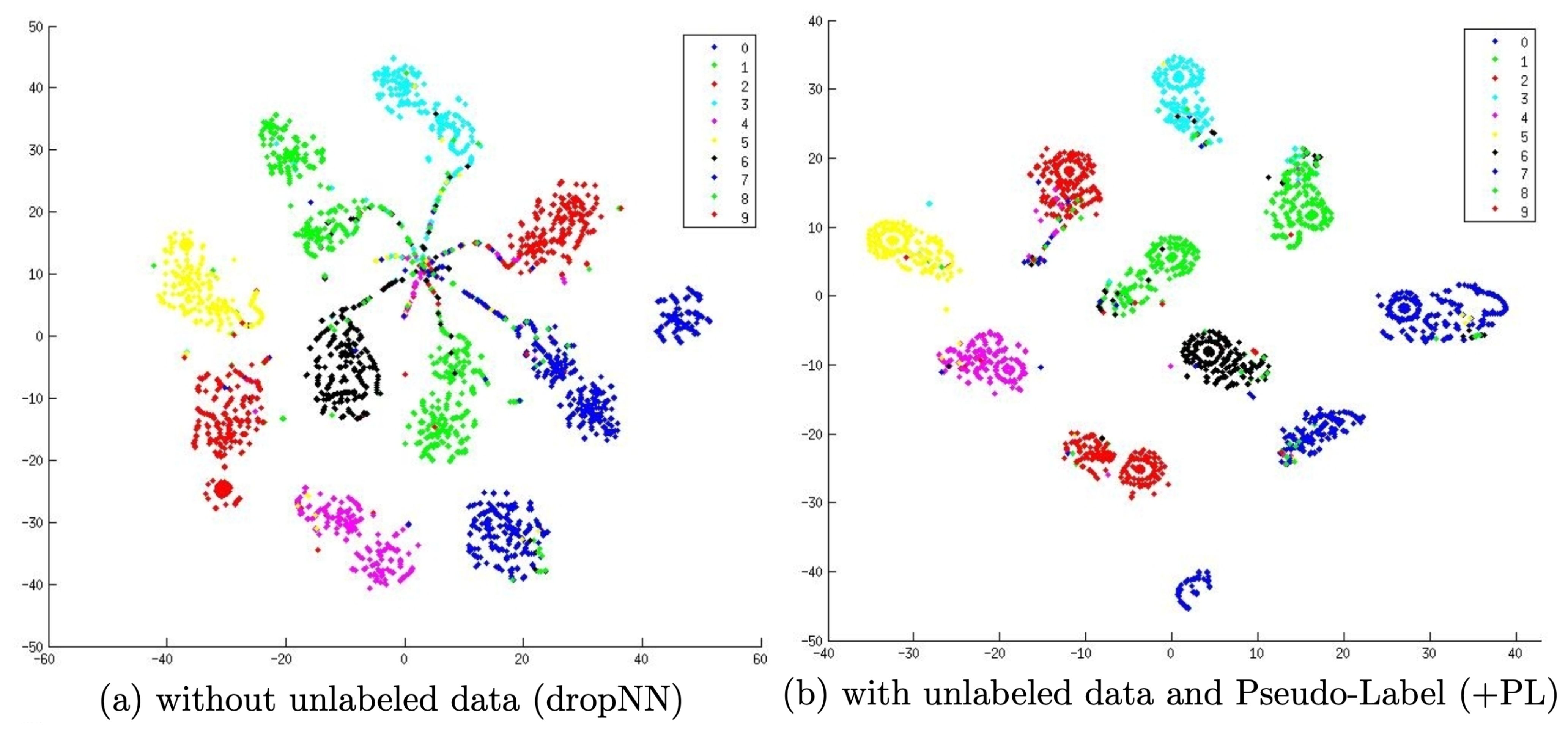
Training with pseudo labeling is naturally iterative. We refer to the model that generates pseudo labels as the teacher, and the model trained on those pseudo labels as the student.
Label propagation
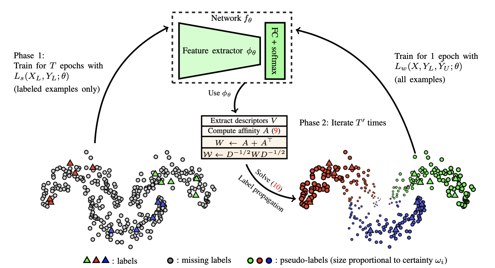
Label Propagation (Iscen et al. 2019) constructs a similarity graph over samples using feature embeddings. Pseudo labels are then “diffused” from labeled samples to unlabeled samples, with propagation weights proportional to pairwise similarity scores in the graph. Conceptually, this resembles a k-NN classifier, and both approaches face scaling challenges on very large datasets.
Self-Training
Self-Training is a long-standing idea (Scudder 1965, Nigram & Ghani CIKM 2000). It is an iterative algorithm that alternates between the following two steps until every unlabeled sample has been assigned a label:
- First, train a classifier using the labeled data.
- Next, use the classifier to predict labels for unlabeled data, then convert the most confident predictions into additional labeled samples.
Xie et al. (2020) applied self-training in deep learning and obtained strong results. For ImageNet classification, they first trained an EfficientNet (Tan & Le 2019) teacher to produce pseudo labels for 300M unlabeled images, and then trained a larger EfficientNet student on both ground-truth labeled images and pseudo labeled images. A key element of their setup is that the student is trained with noise, while the teacher generates pseudo labels without noise. For this reason, the method is called Noisy Student. They use stochastic depth (Huang et al. 2016), dropout, and RandAugment to inject noise into the student. Noise is important for enabling the student to surpass the teacher. The combined noise sources encourage a smoother decision frontier on both labeled and unlabeled data.
Additional important technical configurations for noisy student self-training include:
- The student model should be sufficiently large (that is, larger than the teacher) to accommodate more data.
- Noisy student should be combined with data balancing, which is especially important for balancing the number of pseudo labeled images per class.
- Soft pseudo labels perform better than hard labels.
Noisy student also improves adversarial robustness against an FGSM (Fast Gradient Sign Attack = The attack uses the gradient of the loss w.r.t the input data and adjusts the input data to maximize the loss) attack, even though the model is not explicitly optimized for adversarial robustness.
SentAugment, proposed by Du et al. (2020), targets the case where there is insufficient in-domain unlabeled data for self-training in language. It uses sentence embeddings to retrieve in-domain unlabeled samples from a large corpus and then performs self-training on the retrieved sentences.
Reducing confirmation bias
Confirmation bias arises when an imperfect teacher model provides incorrect pseudo labels. If the student overfits to these incorrect labels, the resulting student model may not improve.
To mitigate confirmation bias, Arazo et al. (2019) introduced two techniques. The first is to apply MixUp with soft labels. Given two samples, $(\mathbf{x}_i, \mathbf{x}_j)$, and their corresponding true or pseudo labels $(y_i, y_j)$, the interpolated-label formulation can be expressed as a cross entropy loss over softmax outputs:
However, MixUp alone is not sufficient when the number of labeled examples is very small. To address this, they enforce a minimum number of labeled samples in every mini-batch by oversampling the labeled data. This strategy outperforms simply upweighting labeled samples because it yields more frequent parameter updates, rather than a smaller number of higher-magnitude updates that may be less stable. As with consistency regularization, strong data augmentation and dropout are also important for pseudo labeling to perform well.
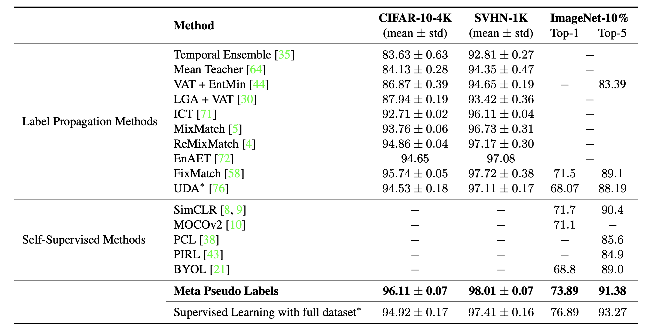
Meta Pseudo Labels (Pham et al. 2021) continuously adapts the teacher model using feedback based on the student’s performance on the labeled dataset. The teacher and student are trained in parallel: the teacher learns to produce higher-quality pseudo labels, and the student learns from those pseudo labels.
Let the teacher and student model weights be $\theta_T$ and $\theta_S$, respectively. Define the student model’s loss on labeled samples as a function $\theta^\text{PL}_S(.)$ of $\theta_T$. The goal is to minimize this loss by optimizing the teacher model accordingly:
Directly optimizing the objective above is not straightforward. Drawing on the idea from MAML, the method approximates the multi-step $\arg\min_{\theta_S}$ using a one-step gradient update of $\theta_S$:
When pseudo labels are soft, the objective above is differentiable. In contrast, hard pseudo labels make the objective non-differentiable, in which case reinforcement learning methods (for example, REINFORCE) are required.
The optimization alternates between training the two models:
- Student model update: Given a batch of unlabeled samples $\{ \mathbf{u} \}$, generate pseudo labels using $f_{\theta_T}(\mathbf{u})$, then optimize $\theta_S$ with one step of SGD: $\theta’_S = \color{green}{\theta_S - \eta_S \cdot \nabla_{\theta_S} \mathcal{L}_u(\theta_T, \theta_S)}$.
- Teacher model update: Given a batch of labeled samples $\{(\mathbf{x}^l, y)\}$, reuse the student’s update to optimize $\theta_T$: $\theta’_T = \theta_T - \eta_T \cdot \nabla_{\theta_T} \mathcal{L}_s ( \color{green}{\theta_S - \eta_S \cdot \nabla_{\theta_S} \mathcal{L}_u(\theta_T, \theta_S)} )$. Additionally, the UDA objective is applied to the teacher model to incorporate consistency regularization.
Pseudo Labeling with Consistency Regularization
These two directions can also be combined, enabling semi-supervised learning that uses both pseudo labeling and consistency training.
MixMatch
MixMatch (Berthelot et al. 2019) is a holistic semi-supervised learning method that leverages unlabeled data by integrating the following components:
- Consistency regularization: Encourage the model to produce identical predictions for perturbed versions of unlabeled samples.
- Entropy minimization: Encourage confident predictions on unlabeled data.
- MixUp augmentation: Encourage linear behavior between examples.
Given a batch of labeled data $\mathcal{X}$ and unlabeled data $\mathcal{U}$, augmented variants are constructed via $\text{MixMatch}(.)$, $\bar{\mathcal{X}}$ and $\bar{\mathcal{U}}$. These variants include augmented samples and guessed labels for unlabeled examples:
Here, $T$ is the sharpening temperature used to reduce overlap among guessed labels, $K$ is the number of augmentations generated per unlabeled example, and $\alpha$ is the MixUp parameter.
For each $\mathbf{u}$, MixMatch creates $K$ augmentations, $\bar{\mathbf{u}}^{(k)} = \text{Augment}(\mathbf{u})$ for $k=1, \dots, K$. The pseudo label is then guessed from their average: $\hat{y} = \frac{1}{K} \sum_{k=1}^K p_\theta(y \mid \bar{\mathbf{u}}^{(k)})$.
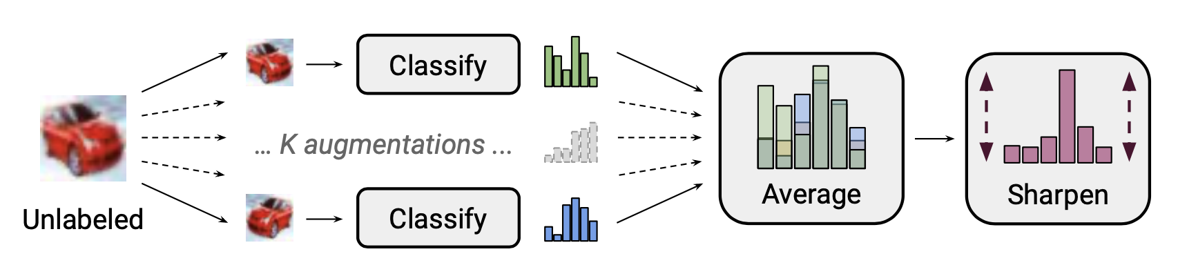
Based on their ablation studies, MixUp is crucial, particularly for unlabeled data. Eliminating temperature sharpening on the pseudo-label distribution substantially degrades performance. Averaging across multiple augmentations during label guessing is also necessary.
ReMixMatch (Berthelot et al. 2020) extends MixMatch with two additional mechanisms:
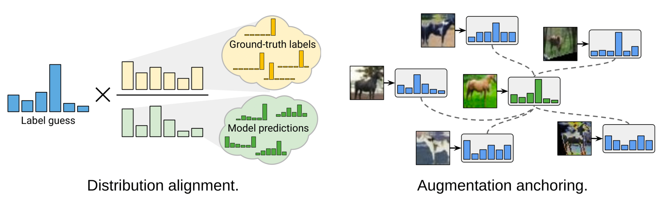
- Distribution alignment. This encourages the marginal distribution $p(y)$ to match the marginal distribution of the ground-truth labels. Let $p(y)$ denote the class distribution over the true labels, and let $\tilde{p}(\hat{y})$ be a running average of the predicted class distribution on unlabeled data. The model prediction for an unlabeled sample $p_\theta(y \vert \mathbf{u})$ is normalized to $\text{Normalize}\big( \frac{p_\theta(y \vert \mathbf{u}) p(y)}{\tilde{p}(\hat{y})} \big)$ to align with the true marginal distribution.
- Note that entropy minimization is not a useful objective when the marginal distribution is not uniform.
- I do feel the assumption that the class distributions on the labeled and unlabeled data should match is too strong and not necessarily to be true in the real-world setting.
- Augmentation anchoring. For each unlabeled sample, the method first generates an “anchor” view using weak augmentation, then averages $K$ strongly augmented views produced with CTAugment (Control Theory Augment). CTAugment samples only augmentations that keep the model predictions within the network tolerance.
The ReMixMatch loss combines multiple terms:
- a supervised loss with data augmentation and MixUp applied;
- an unsupervised loss with data augmentation and MixUp applied, using pseudo labels as targets;
- a CE loss on a single heavily-augmented unlabeled image without MixUp;
- a rotation loss as in self-supervised learning.
DivideMix
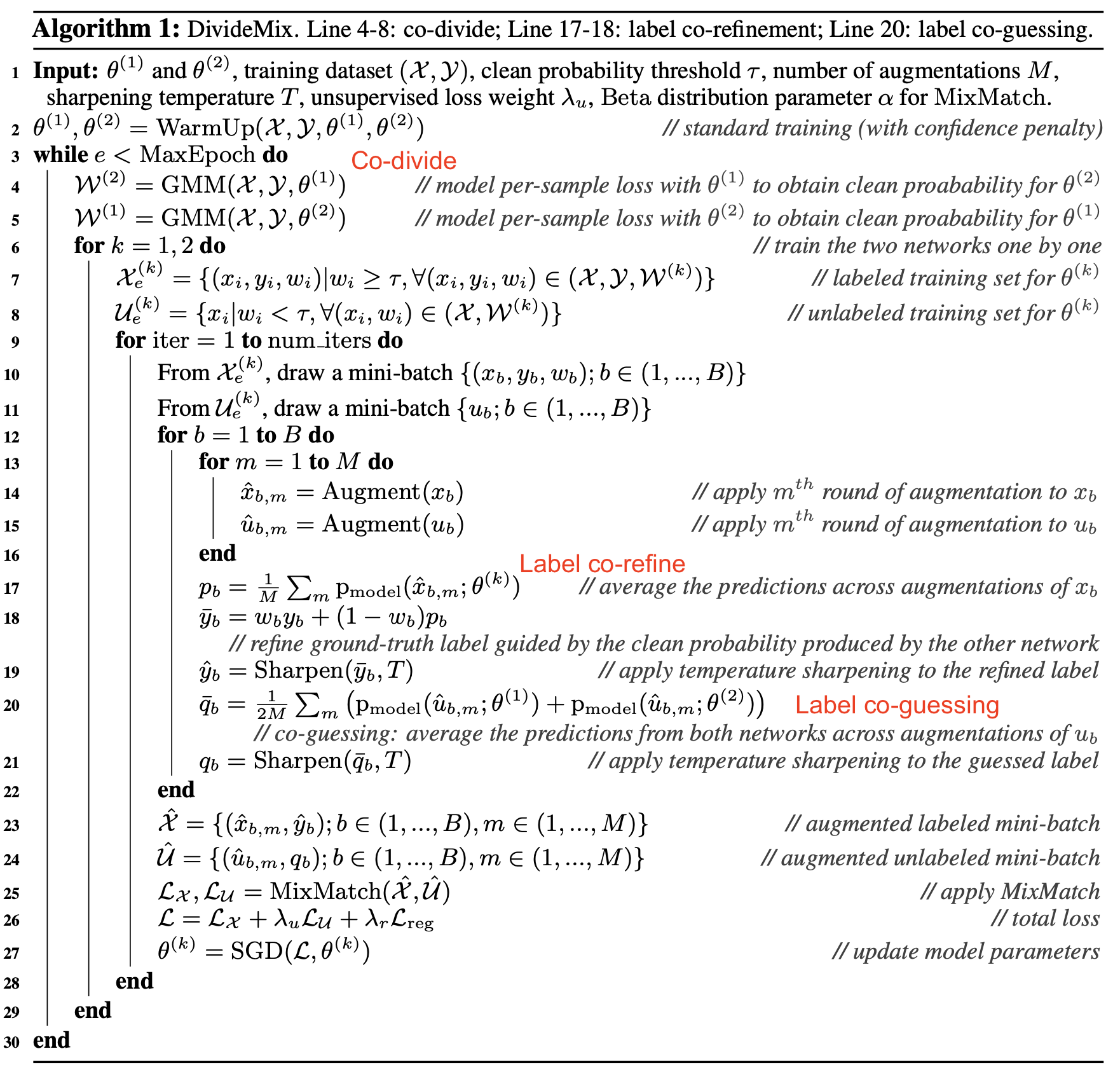
DivideMix (Junnan Li et al. 2020) combines semi-supervised learning with Learning with noisy labels (LNL). It models the per-sample loss distribution using a GMM, enabling dynamic partitioning of the training data into a labeled set of clean examples and an unlabeled set of noisy examples. Following Arazo et al. 2019, they fit a two-component GMM to the per-sample cross entropy loss $\ell_i = y_i^\top \log f_\theta(\mathbf{x}_i)$. Clean samples are expected to reach low loss values faster than noisy samples. The component with the smaller mean is treated as the clean-label cluster, denoted $c$. If the GMM posterior probability $w_i = p_\text{GMM}(c \mid \ell_i)$ (that is, the probability that the sample belongs to the clean set) exceeds the threshold $\tau$, the sample is treated as clean; otherwise, it is treated as noisy.
This clustering step is referred to as co-divide. To reduce confirmation bias, DivideMix trains two diverged networks simultaneously, where each network uses the data split produced by the other, analogous to the intuition behind Double Q Learning.
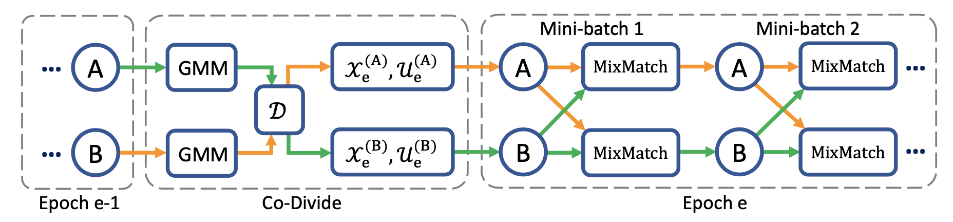
Relative to MixMatch, DivideMix introduces an explicit co-divide phase to handle noisy samples, and it also adds the following training refinements:
- Label co-refinement: It linearly combines the ground-truth label $y_i$ with the network’s prediction $\hat{y}_i$. The prediction is averaged over multiple augmentations of $\mathbf{x}_i$ and is weighted using the clean-set probability $w_i$ produced by the other network.
- Label co-guessing: It averages predictions from the two models for unlabeled samples.
FixMatch
FixMatch (Sohn et al. 2020) produces pseudo labels for unlabeled samples using weak augmentation and retains only high-confidence predictions. Both weak augmentation and confidence-based filtering contribute to more reliable pseudo-label targets. FixMatch then trains the model to predict these pseudo labels from heavily augmented inputs.
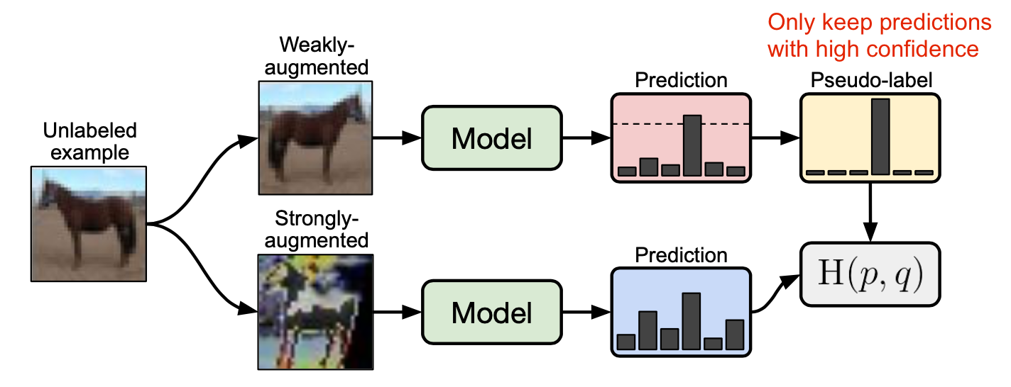
where $\hat{y}_b$ is the pseudo label for an unlabeled example, and $\mu$ is a hyperparameter controlling the relative sizes of $\mathcal{X}$ and $\mathcal{U}$.
- Weak augmentation $\mathcal{A}_\text{weak}(.)$: A standard flip-and-shift augmentation
- Strong augmentation $\mathcal{A}_\text{strong}(.)$ : AutoAugment, Cutout, RandAugment, CTAugment
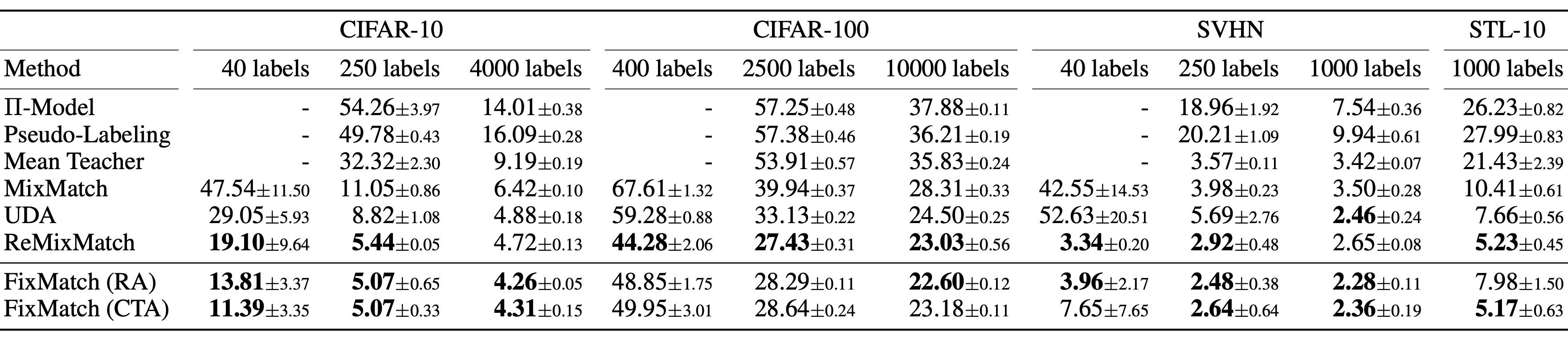
The FixMatch ablation studies report the following:
- Sharpening the predicted distribution with a temperature parameter $T$ has no significant effect when the threshold $\tau$ is used.
- Cutout and CTAugment, as part of the strong augmentation pipeline, are required for good performance.
- If the weak augmentation used for label guessing is replaced with strong augmentation, training diverges early. If weak augmentation is removed entirely, the model overfits to the guessed labels.
- Using weak rather than strong augmentation for pseudo-label prediction yields unstable results. Strong data augmentation is essential.
Combined with Powerful Pre-Training
A common paradigm, particularly for language tasks, is to first pre-train a task-agnostic model on a large unlabeled corpus via self-supervised learning, then fine-tune it on a downstream task using a small labeled dataset. Research indicates that additional gains are possible when semi-supervised learning is combined with pre-training.
Zoph et al. (2020) investigated when self-training can be more effective than pre-training. Their experimental setup used ImageNet for either pre-training or self-training to improve COCO performance. Note that when ImageNet is used for self-training, labels are discarded and ImageNet examples are treated only as unlabeled data. He et al. (2018) showed that ImageNet classification pre-training performs poorly when the downstream task differs substantially, such as object detection.
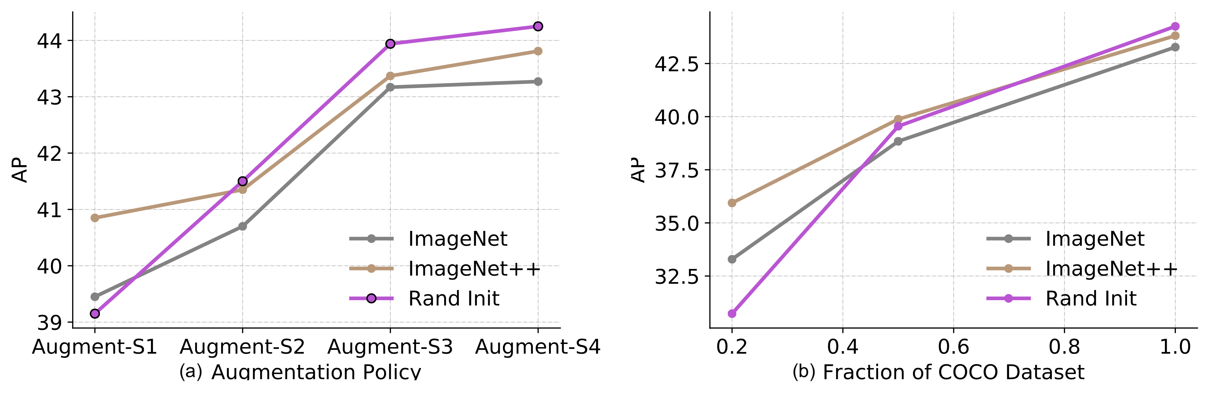
Their experiments highlighted several notable findings:
- The benefit of pre-training decreases as more labeled downstream data becomes available. Pre-training helps in low-data regimes (20%) but is neutral or harmful in high-data regimes.
- Self-training is beneficial in high-data and strong-augmentation regimes, including cases where pre-training is detrimental.
- Self-training can provide additive improvements on top of pre-training, even when both use the same data source.
- Self-supervised pre-training (for example, SimCLR) reduces performance in high-data regimes, similar to supervised pre-training.
- Joint training with supervised and self-supervised objectives helps mitigate mismatch between the pre-training task and the downstream task. Pre-training, joint-training, and self-training are additive.
- Noisy labels or un-targeted labeling (that is, pre-training labels not aligned with downstream task labels) performs worse than targeted pseudo labeling.
- Self-training is computationally more expensive than fine-tuning from a pre-trained model.
Chen et al. (2020) proposed a three-step procedure that combines the advantages of self-supervised pretraining, supervised fine-tuning, and self-training:
- Pre-train a large model using an unsupervised or self-supervised objective.
- Fine-tune the model in a supervised manner using a small labeled set. Using a large (deep and wide) neural network is important. Bigger models yield better performance with fewer labeled samples.
- Perform distillation with unlabeled examples by adopting pseudo labels in self-training.
- Knowledge can be distilled from a large model into a smaller model because task-specific deployment does not require additional representational capacity.
- The distillation loss is defined as follows, with a fixed teacher network having weights $\hat{\theta}_T$.
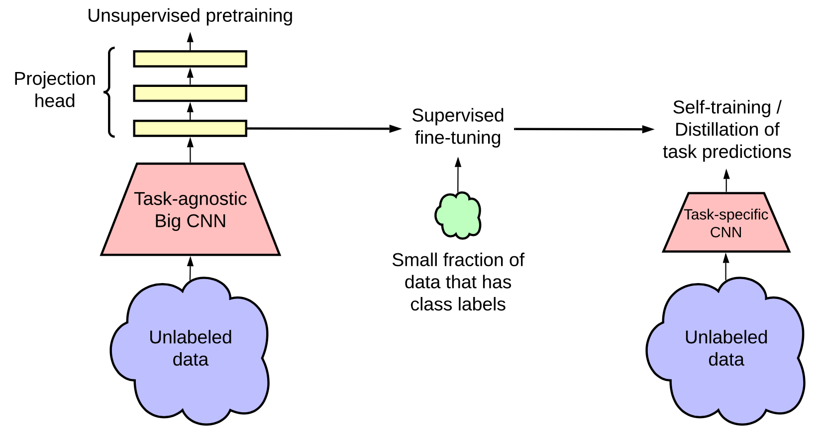
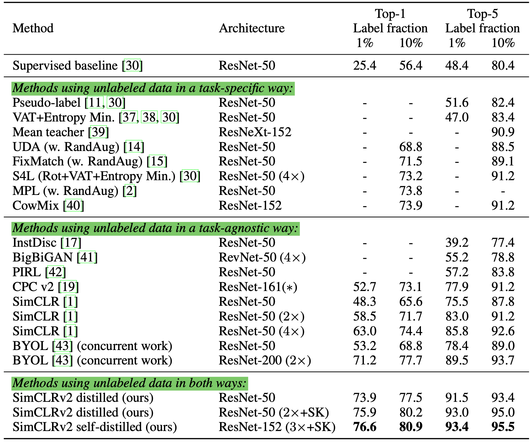
They evaluated this approach on ImageNet classification. The self-supervised pre-training component uses SimCLRv2, a direct improvement over SimCLR. Their empirical results support several conclusions that align with Zoph et al. 2020:
- Bigger models are more label-efficient;
- Bigger/deeper project heads in SimCLR improve representation learning;
- Distillation using unlabeled data improves semi-supervised learning.
💡 Quick summary of common themes among recent semi-supervised learning methods, many aiming to reduce confirmation bias:
- Apply valid and diverse noise to samples via advanced data augmentation methods.
- For image tasks, MixUp is an effective augmentation. MixUp may also be applicable to language, yielding a small incremental improvement (Guo et al. 2019).
- Use a confidence threshold and discard low-confidence pseudo labels.
- Enforce a minimum number of labeled samples per mini-batch.
- Sharpen the pseudo-label distribution to reduce class overlap.
Citation
Cited as:
Weng, Lilian. (Dec 2021). Learning with not enough data part 1: semi-supervised learning. Lil’Log. https://lilianweng.github.io/posts/2021-12-05-semi-supervised/.
Or
@article{weng2021semi,
  title   = "Learning with not Enough Data Part 1: Semi-Supervised Learning",
  author  = "Weng, Lilian",
  journal = "lilianweng.github.io",
  year    = "2021",
  month   = "Dec",
  url     = "https://lilianweng.github.io/posts/2021-12-05-semi-supervised/"
}
References
[1] Ouali, Hudelot & Tami. “An Overview of Deep Semi-Supervised Learning” arXiv preprint arXiv:2006.05278 (2020).
[2] Sajjadi, Javanmardi & Tasdizen “Regularization With Stochastic Transformations and Perturbations for Deep Semi-Supervised Learning.” arXiv preprint arXiv:1606.04586 (2016).
[3] Pham et al. “Meta Pseudo Labels.” CVPR 2021.
[4] Laine & Aila. “Temporal Ensembling for Semi-Supervised Learning” ICLR 2017.
[5] Tarvaninen & Valpola. “Mean teachers are better role models: Weight-averaged consistency targets improve semi-supervised deep learning results.” NeuriPS 2017
[6] Xie et al. “Unsupervised Data Augmentation for Consistency Training.” NeuriPS 2020.
[7] Miyato et al. “Virtual Adversarial Training: A Regularization Method for Supervised and Semi-Supervised Learning.” IEEE transactions on pattern analysis and machine intelligence 41.8 (2018).
[8] Verma et al. “Interpolation consistency training for semi-supervised learning.” IJCAI 2019
[9] Lee. “Pseudo-label: The simple and efficient semi-supervised learning method for deep neural networks.” ICML 2013 Workshop: Challenges in Representation Learning.
[10] Iscen et al. “Label propagation for deep semi-supervised learning.” CVPR 2019.
[11] Xie et al. “Self-training with Noisy Student improves ImageNet classification” CVPR 2020.
[12] Jingfei Du et al. “Self-training Improves Pre-training for Natural Language Understanding.” 2020
[13] Iscen et al. “Label propagation for deep semi-supervised learning.” CVPR 2019
[14] Arazo et al. “Pseudo-labeling and confirmation bias in deep semi-supervised learning.” IJCNN 2020.
[15] Berthelot et al. “MixMatch: A holistic approach to semi-supervised learning.” NeuriPS 2019
[16] Berthelot et al. “ReMixMatch: Semi-supervised learning with distribution alignment and augmentation anchoring.” ICLR 2020
[17] Sohn et al. “FixMatch: Simplifying semi-supervised learning with consistency and confidence.” CVPR 2020
[18] Junnan Li et al. “DivideMix: Learning with Noisy Labels as Semi-supervised Learning.” 2020 [code]
[19] Zoph et al. “Rethinking pre-training and self-training.” 2020.
[20] Chen et al. “Big Self-Supervised Models are Strong Semi-Supervised Learners” 2020