This tutorial walks through building a recurrent neural network in TensorFlow for stock market price prediction. The full working code is available at github.com/lilianweng/stock-rnn. If you are not yet familiar with recurrent neural networks or LSTM cells, you can review my previous post.

One point I want to highlight: my primary motivation for writing this post is to demonstrate how to build and train an RNN model in TensorFlow, rather than to thoroughly solve the stock prediction problem. As a result, I did not put significant effort into improving prediction performance. You are very welcome to use my code as a baseline and incorporate additional stock-prediction ideas to improve it. Enjoy!

Overview of Existing Tutorials

There are many tutorials available online, such as:

• A noob’s guide to implementing RNN-LSTM using Tensorflow
• TensorFlow RNN Tutorial
• LSTM by Example using Tensorflow
• How to build a Recurrent Neural Network in TensorFlow
• RNNs in Tensorflow, a Practical Guide and Undocumented Features
• Sequence prediction using recurrent neural networks(LSTM) with TensorFlow
• Anyone Can Learn To Code an LSTM-RNN in Python
• How to do time series prediction using RNNs, TensorFlow and Cloud ML Engine

Even with these resources, I still wanted to write another tutorial, mainly for three reasons:

1. Many early tutorials no longer work well with newer releases, because TensorFlow is still evolving and its API interfaces change quickly.
2. A lot of tutorials rely on synthetic data in their examples, while I wanted to work with real-world data.
3. Some tutorials assume prior familiarity with the TensorFlow API, which can make them harder to follow.

After reviewing many examples, I recommend using the official example on the Penn Tree Bank (PTB) dataset as a starting point. The PTB example presents an RNN model using a clean, modular design pattern, but that structure can make the model itself harder to understand at first. For that reason, I will build the graph here in a more direct and explicit way.

The Goal

I will explain how to construct an RNN model with LSTM cells to predict S&P500 index prices. The dataset can be downloaded from Yahoo! Finance ^GSPC. In the example below, I used S&P 500 data from Jan 3, 1950 (the earliest date Yahoo! Finance can trace back to) through Jun 23, 2017. The dataset includes multiple price points per day; for simplicity, we use only the daily close prices for prediction. I will also demonstrate how to use TensorBoard to simplify debugging and track model behavior.

As a quick recap: a recurrent neural network (RNN) is a type of artificial neural network that includes self-loops in its hidden layer(s). This structure allows an RNN to use the previous hidden state to learn the current state given a new input, making it well suited for sequential data. A long short-term memory (LSTM) cell is a specialized unit designed to help an RNN retain long-term context more effectively.

For a deeper discussion, please refer to my previous post or this awesome post.

Data Preparation

The stock prices form a time series of length $N$, defined as $p_0, p_1, \dots, p_{N-1}$, where $p_i$ is the closing price on day $i$, $0 \le i < N$. Consider a sliding window with fixed size $w$ (later referred to as input_size). Each time, we shift the window to the right by $w$, ensuring there is no overlap across the sliding windows.

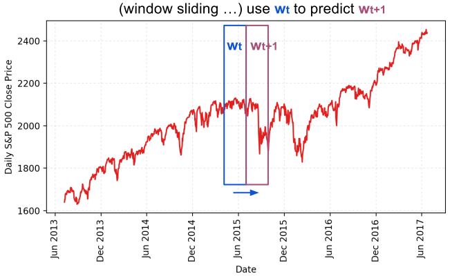
The RNN model we will build uses LSTM cells as the basic hidden units. We take values starting from the beginning of the first sliding window $W_0$ through the window $W_t$ at time $t$:

and use them to predict the prices in the next window $w_{t+1}$:

$ W_{t+1} = (p_{(t+1)w}, p_{(t+1)w+1}, \dots, p_{(t+2)w-1}) $

In other words, we aim to learn an approximation function, $f(W_0, W_1, \dots, W_t) \approx W_{t+1}$.

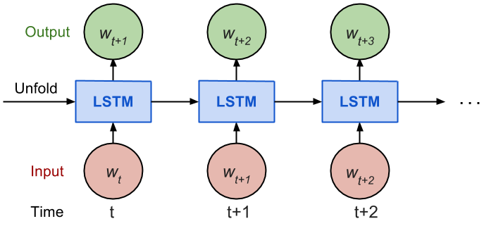
Given how back propagation through time (BPTT) works, RNNs are commonly trained in an “unrolled” form. This avoids propagating gradients too far back in time and reduces training complexity.

Below is TensorFlow’s explanation of num_steps from Tensorflow’s tutorial:

By design, the output of a recurrent neural network (RNN) depends on arbitrarily distant inputs. Unfortunately, this makes backpropagation computation difficult. In order to make the learning process tractable, it is common practice to create an “unrolled” version of the network, which contains a fixed number (num_steps) of LSTM inputs and outputs. The model is then trained on this finite approximation of the RNN. This can be implemented by feeding inputs of length num_steps at a time and performing a backward pass after each such input block.

We first split the price sequence into small, non-overlapping windows. Each window contains input_size numbers and is treated as one independent input element. Next, we group any num_steps consecutive input elements into a single training input, creating an “un-rolled” RNN representation for training in Tensorfow. The corresponding label is the input element immediately following that group.

For example, with input_size=3 and num_steps=2, the first few training examples would be:

The key code for formatting the data is shown below:

seq = [np.array(seq[i * self.input_size: (i + 1) * self.input_size]) 
       for i in range(len(seq) // self.input_size)]

# Split into groups of `num_steps`
X = np.array([seq[i: i + self.num_steps] for i in range(len(seq) - self.num_steps)])
y = np.array([seq[i + self.num_steps] for i in range(len(seq) - self.num_steps)])

The complete data-formatting code is available here.

Train / Test Split

Because the objective is always to predict future values, we reserve the latest 10% of the data as the test set.

Normalization

The S&P 500 index rises over time, which creates a scaling issue: most values in the test set end up outside the range of the training set, meaning the model must predict numbers it has never seen before. Unsurprisingly, the result is poor. See

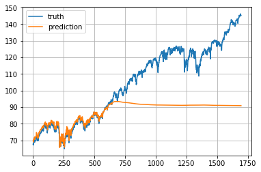
To address this out-of-scale problem, I normalize the prices within each sliding window. This reframes the task as predicting relative change rates rather than absolute values. In a normalized sliding window $W’_t$ at time $t$, each value is divided by the last unknown price, namely the final price in $W_{t-1}$:

$ W’_t = (\frac{p_{tw}}{p_{tw-1}}, \frac{p_{tw+1}}{p_{tw-1}}, \dots, \frac{p_{(t+1)w-1}}{p_{tw-1}}) $

Here is a data archive, stock-data-lilianweng.tar.gz, containing S & P 500 stock prices that I crawled up to Jul, 2017. Feel free to play with it :)

Model Construction

Definitions

• lstm_size: the number of units in one LSTM layer.
• num_layers: the number of stacked LSTM layers.
• keep_prob: the proportion of cell units retained during the dropout operation.
• init_learning_rate: the initial learning rate.
• learning_rate_decay: the decay ratio used in later training epochs.
• init_epoch: the number of epochs trained with constant init_learning_rate.
• max_epoch: the total number of training epochs.
• input_size: the size of the sliding window (one training data point).
• batch_size: the number of data points per mini-batch.

The LSTM model includes num_layers stacked LSTM layer(s), and each layer contains lstm_size LSTM cells. A dropout mask with keep probability keep_prob is applied to the output of every LSTM cell. Dropout is intended to reduce excessive reliance on any single dimension and thus help prevent overfitting.

Training runs for max_epoch epochs in total. An epoch is one complete pass over all training data points. During each epoch, the training data is divided into mini-batches of size batch_size. Each mini-batch is fed into the model for one BPTT update. The learning rate remains init_learning_rate for the first init_epoch epochs, and then it decays by $\times$ learning_rate_decay in every subsequent epoch.

# Configuration is wrapped in one object for easy tracking and passing.
class RNNConfig():
    input_size=1
    num_steps=30
    lstm_size=128
    num_layers=1
    keep_prob=0.8
    batch_size = 64
    init_learning_rate = 0.001
    learning_rate_decay = 0.99
    init_epoch = 5
    max_epoch = 50

config = RNNConfig()

Define Graph

A tf.Graph is not bound to any concrete data. Instead, it specifies how data will be processed and how computations will be executed. Later, you can feed real data into the graph within a tf.session, at which point the computation is actually carried out.

Let’s walk through the code.

(1) First, initialize a new graph.

import tensorflow as tf
tf.reset_default_graph()
lstm_graph = tf.Graph()

(2) Define the graph behavior within its scope.

with lstm_graph.as_default():

(3) Specify the inputs required for computation. We need three input variables, each created using tf.placeholder because their values are unknown during graph construction.

• inputs: the training data X, a tensor with shape (# data examples, num_steps, input_size). The number of examples is unknown at graph-build time, so it is set to None. In our case, it will be batch_size during training. If this is unclear, refer to the input format example.
• targets: the training label y, a tensor with shape (# data examples, input_size).
• learning_rate: a scalar float.

    # Dimension = (
    #     number of data examples, 
    #     number of input in one computation step, 
    #     number of numbers in one input
    # )
    # We don't know the number of examples beforehand, so it is None.
    inputs = tf.placeholder(tf.float32, [None, config.num_steps, config.input_size])
    targets = tf.placeholder(tf.float32, [None, config.input_size])
    learning_rate = tf.placeholder(tf.float32, None)

(4) This function returns a single LSTMCell, optionally with dropout applied.

    def _create_one_cell():
        return tf.contrib.rnn.LSTMCell(config.lstm_size, state_is_tuple=True)
        if config.keep_prob < 1.0:
            return tf.contrib.rnn.DropoutWrapper(lstm_cell, output_keep_prob=config.keep_prob)

(5) Stack multiple cells into multiple layers when needed. MultiRNNCell connects multiple simple cells sequentially to form a composite cell.

    cell = tf.contrib.rnn.MultiRNNCell(
        [_create_one_cell() for _ in range(config.num_layers)], 
        state_is_tuple=True
    ) if config.num_layers > 1 else _create_one_cell()

(6) tf.nn.dynamic_rnn builds a recurrent neural network defined by cell (an RNNCell). It returns a pair, (model outputs, state). By default, the outputs val have shape (batch_size, num_steps, lstm_size). The state is the current LSTM cell state and is not used here.

    val, _ = tf.nn.dynamic_rnn(cell, inputs, dtype=tf.float32)

(7) tf.transpose changes the output dimensions from (batch_size, num_steps, lstm_size) to (num_steps, batch_size, lstm_size). We then select the final output.

    # Before transpose, val.get_shape() = (batch_size, num_steps, lstm_size)
    # After transpose, val.get_shape() = (num_steps, batch_size, lstm_size)
    val = tf.transpose(val, [1, 0, 2])
    # last.get_shape() = (batch_size, lstm_size)
    last = tf.gather(val, int(val.get_shape()[0]) - 1, name="last_lstm_output")

(8) Define the weights and biases between the hidden layer and the output layer.

    weight = tf.Variable(tf.truncated_normal([config.lstm_size, config.input_size]))
    bias = tf.Variable(tf.constant(0.1, shape=[config.input_size]))
    prediction = tf.matmul(last, weight) + bias

(9) Use mean squared error as the loss function, and apply the RMSPropOptimizer algorithm for gradient descent optimization.

    loss = tf.reduce_mean(tf.square(prediction - targets))
    optimizer = tf.train.RMSPropOptimizer(learning_rate)
    minimize = optimizer.minimize(loss)

Start Training Session

(1) To train the graph on real data, you must first create a tf.session.

with tf.Session(graph=lstm_graph) as sess:

(2) Initialize the variables according to the definitions in the graph.

    tf.global_variables_initializer().run()

(0) Learning rates for the training epochs should be computed in advance. The index corresponds to the epoch index.

learning_rates_to_use = [
    config.init_learning_rate * (
        config.learning_rate_decay ** max(float(i + 1 - config.init_epoch), 0.0)
    ) for i in range(config.max_epoch)]

(3) Each iteration of the loop below performs training for one full epoch.

    for epoch_step in range(config.max_epoch):
        current_lr = learning_rates_to_use[epoch_step]
        
        # Check https://github.com/lilianweng/stock-rnn/blob/master/data_wrapper.py
        # if you are curious to know what is StockDataSet and how generate_one_epoch() 
        # is implemented.
        for batch_X, batch_y in stock_dataset.generate_one_epoch(config.batch_size):
            train_data_feed = {
                inputs: batch_X, 
                targets: batch_y, 
                learning_rate: current_lr
            }
            train_loss, _ = sess.run([loss, minimize], train_data_feed)

(4) Remember to save the trained model when training finishes.

    saver = tf.train.Saver()
    saver.save(sess, "your_awesome_model_path_and_name", global_step=max_epoch_step)

The full code listing is available here.

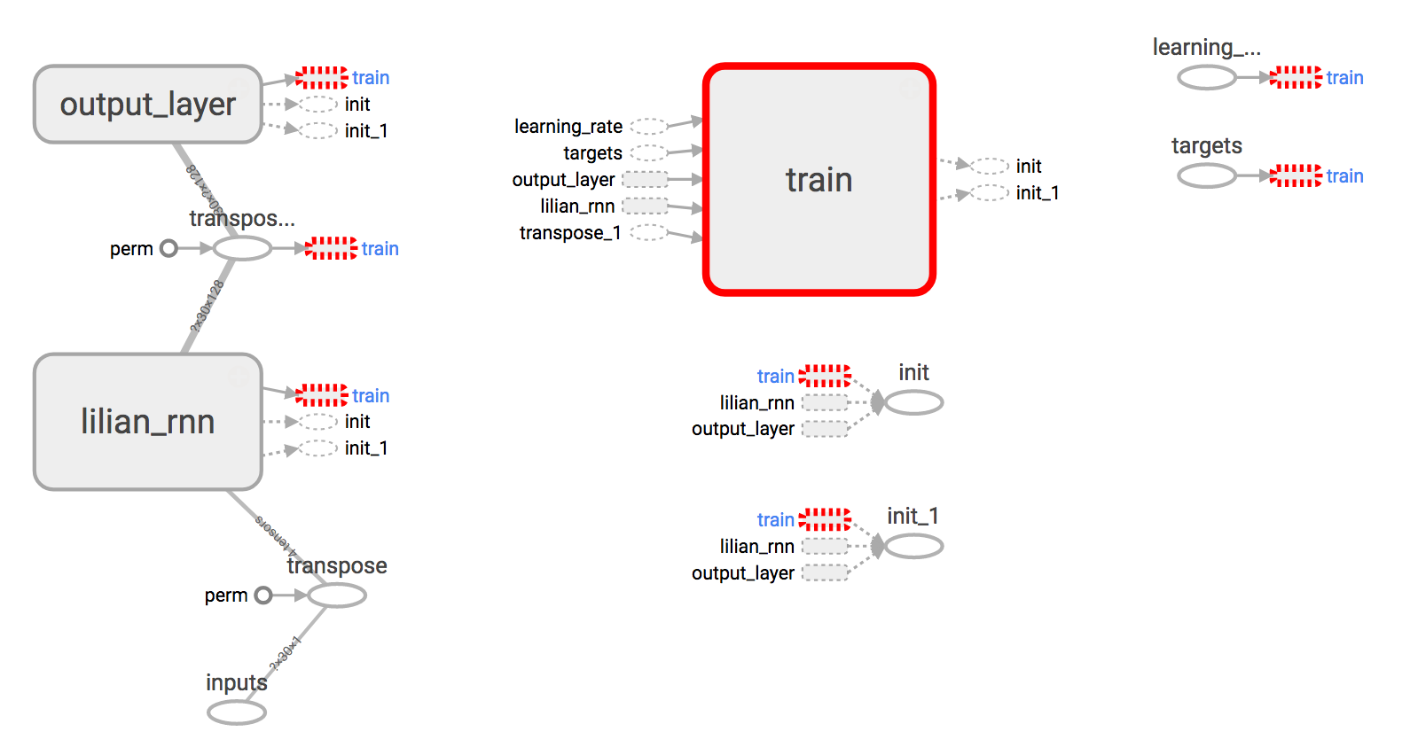
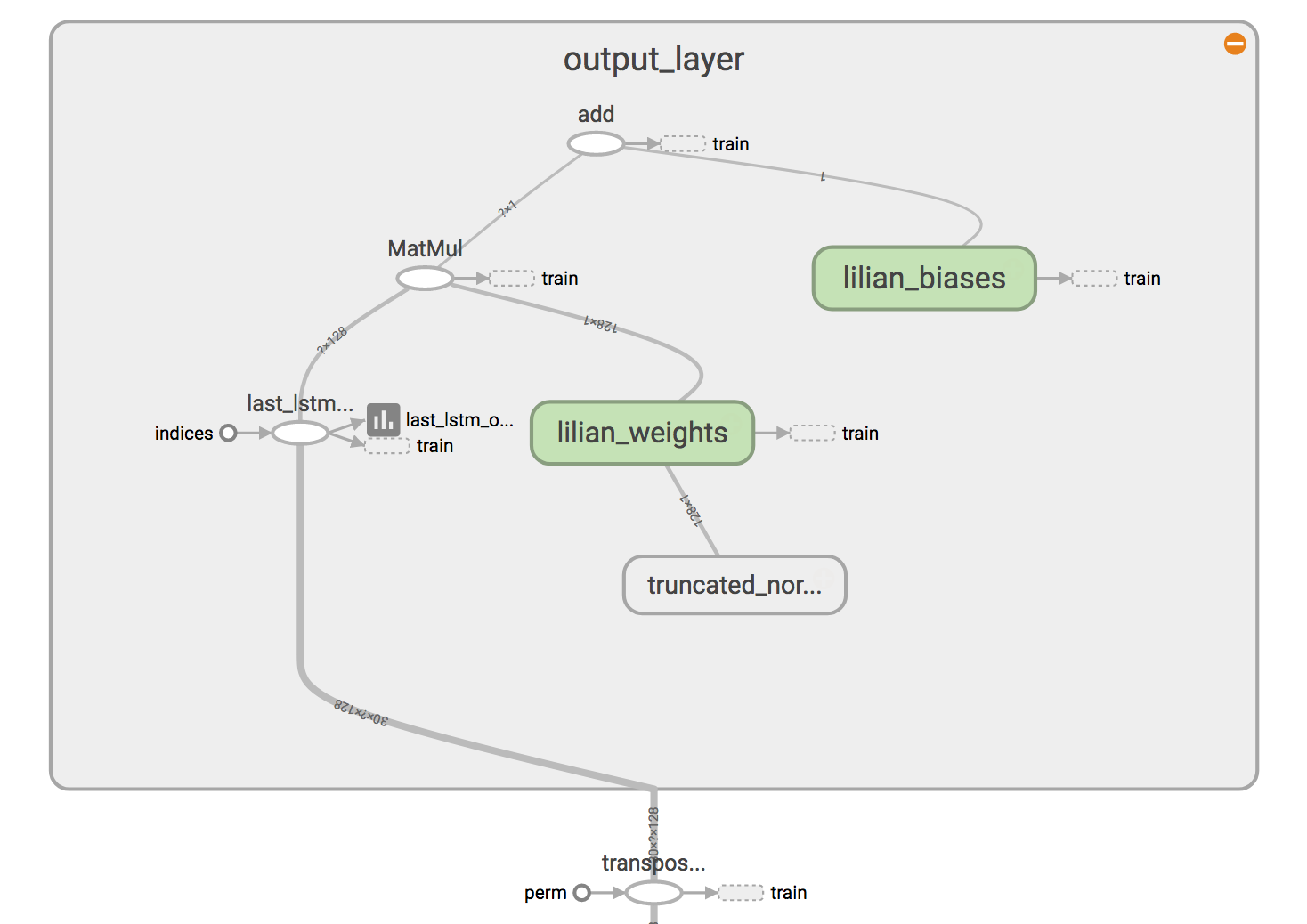
Use TensorBoard

Constructing a graph without visualization is comparable to drawing in the dark: it is difficult to interpret and easy to get wrong. Tensorboard offers convenient visualizations for both the graph structure and the learning dynamics. See this hand-on tutorial; it is only 20 minutes long, yet highly practical, and it demonstrates several live examples.

Brief Summary

• Use with [tf.name_scope](https://www.tensorflow.org/api_docs/python/tf/name_scope)("your_awesome_module_name"): to group elements that serve the same objective.
• Many tf.* methods accept a name= argument. Providing explicit, custom names makes the graph substantially easier to read and navigate.
• Functions such as tf.summary.scalar and tf.summary.histogram allow you to monitor variable values in the graph over iterations.
• Within the training session, configure a log file via tf.summary.FileWriter.

with tf.Session(graph=lstm_graph) as sess:
    merged_summary = tf.summary.merge_all()
    writer = tf.summary.FileWriter("location_for_keeping_your_log_files", sess.graph)
    writer.add_graph(sess.graph)

Then, write training progress and summary outputs to the file.

_summary = sess.run([merged_summary], test_data_feed)
writer.add_summary(_summary, global_step=epoch_step)  # epoch_step in range(config.max_epoch)

The complete, runnable code is available at github.com/lilianweng/stock-rnn.

Results

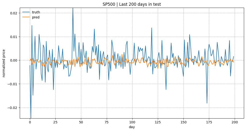
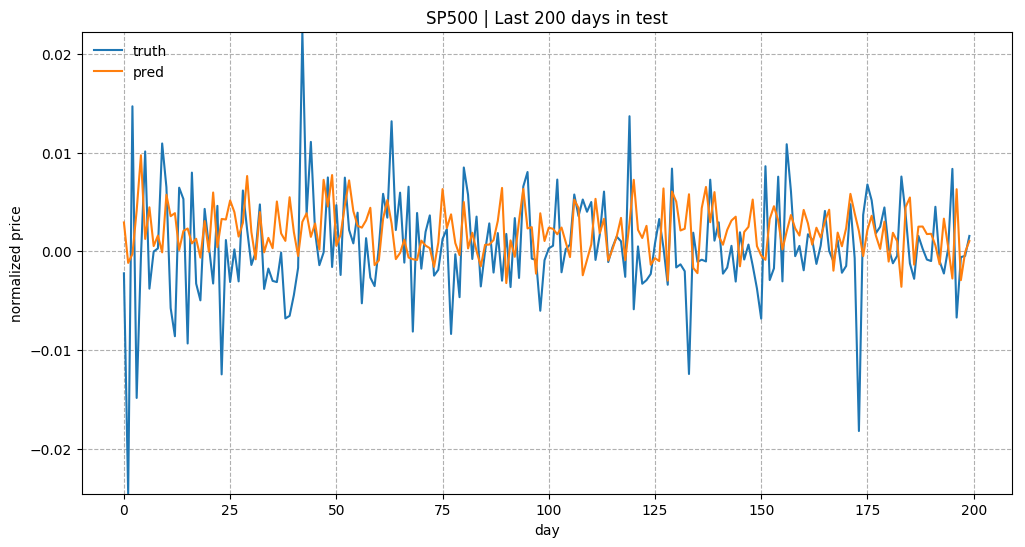
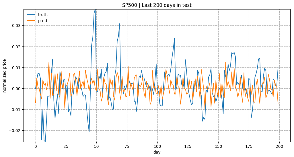
I ran the experiment using the configuration below.

num_layers=1
keep_prob=0.8
batch_size = 64
init_learning_rate = 0.001
learning_rate_decay = 0.99
init_epoch = 5
max_epoch = 100
num_steps=30

(Thanks to Yury for cathcing a bug in the price normalization. Rather than using the last price from the previous time window, I mistakenly used the last price from the same window. The plots below have been corrected.)

In general, predicting stock prices is challenging. After normalization in particular, the price trajectories appear very noisy.

The tutorial’s example code is available at github.com/lilianweng/stock-rnn:scripts.

(Updated on Sep 14, 2017) The model implementation has been updated and is now wrapped in a class: LstmRNN. Model training can be launched from main.py, for example:

python main.py --stock_symbol=SP500 --train --input_size=1 --lstm_size=128