In Part 2, I continue the stock price prediction topic and extend the recurrent neural network built in Part 1 so that it can handle multiple stocks. To help the model differentiate patterns across different price sequences, I incorporate stock symbol embedding vectors as part of the input.

Dataset

While researching, I found this library for querying the Yahoo! Finance API. It would have been very helpful if Yahoo had not shut down the historical data fetch API. However, you may still find it useful for querying other types of information. Here, I use the Google Finance link, selected from a couple of free data sources, to download historical stock prices.

The data-fetching code can be as simple as:

import urllib2
from datetime import datetime
BASE_URL = "https://www.google.com/finance/historical?"
           "output=csv&q={0}&startdate=Jan+1%2C+1980&enddate={1}"
symbol_url = BASE_URL.format(
    urllib2.quote('GOOG'), # Replace with any stock you are interested.
    urllib2.quote(datetime.now().strftime("%b+%d,+%Y"), '+')
)

When retrieving content, remember to include a try-catch wrapper in case the link fails or the supplied stock symbol is invalid.

try:
    f = urllib2.urlopen(symbol_url)
    with open("GOOG.csv", 'w') as fin:
        print >> fin, f.read()
except urllib2.HTTPError:
    print "Fetching Failed: {}".format(symbol_url)

The full, working data fetcher implementation is available at here.

Model Construction

The model is intended to learn, over time, the price sequences of different stocks. Because the underlying patterns vary by stock, I want to explicitly indicate which stock the model is processing. Embedding is preferable to one-hot encoding for the following reasons:

1. If the training set contains $N$ stocks, one-hot encoding would add $N$ (or $N-1$) additional sparse feature dimensions. By mapping each stock symbol to a much smaller embedding vector of length $k$, $k \ll N$, we obtain a far more compact representation and a smaller dataset to manage.
2. Embedding vectors are learned variables. Similar stocks can end up with similar embeddings, which can improve each other’s predictions, for example, “GOOG” and “GOOGL”, as shown later.

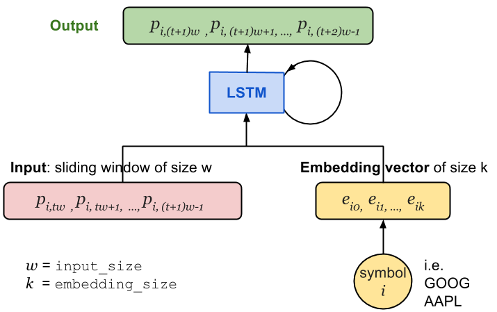
In the recurrent neural network, at time step $t$, the input vector contains input_size (labeled as $w$) daily price values of the $i$-th stock, $(p_{i, tw}, p_{i, tw+1}, \dots, p_{i, (t+1)w-1})$. The stock symbol is uniquely mapped to a vector of length embedding_size (labeled as $k$), $(e_{i,0}, e_{i,1}, \dots, e_{i,k})$. As shown in Fig. 1., the price vector is concatenated with the embedding vector and then fed into the LSTM cell.

An alternative approach is to concatenate the embedding vectors with the final LSTM state, then learn new weights $W$ and bias $b$ in the output layer. However, under that design, the LSTM cell itself cannot distinguish one stock’s prices from another’s, and its capacity would be significantly constrained. Therefore, I use the former approach.

Two new configuration settings are added to RNNConfig:

• embedding_size controls the dimensionality of each embedding vector.
• stock_count specifies the number of unique stocks in the dataset.

Together, these determine the shape of the embedding matrix. As a result, compared with the model in Part 1, the model must learn embedding_size $\times$ stock_count additional variables.

class RNNConfig():
   # ... old ones
   embedding_size = 3
   stock_count = 50

Define the Graph

, Let’s start going through some code ,

(1) As shown in tutorial Part 1: Define the Graph, we define a tf.Graph() named lstm_graph and create tensors to hold input data, inputs, targets, and learning_rate, using the same approach. We also need one additional placeholder: a list of stock symbols associated with the input prices. The stock symbols have been mapped to unique integers in advance using label encoding.

# Mapped to an integer. one label refers to one stock symbol.
stock_labels = tf.placeholder(tf.int32, [None, 1])

(2) Next, we create an embedding matrix to serve as a lookup table that holds the embedding vectors for all stocks. The matrix is initialized with random values in the interval [-1, 1] and is updated during training.

# NOTE: config = RNNConfig() and it defines hyperparameters.
# Convert the integer labels to numeric embedding vectors.
embedding_matrix = tf.Variable(
    tf.random_uniform([config.stock_count, config.embedding_size], -1.0, 1.0)
)

(3) Repeat the stock labels num_steps times so they match the unfolded RNN representation and the shape of the inputs tensor during training. The transformation operation tf.tile takes a base tensor and produces a new tensor by replicating certain dimensions multiple times. Specifically, the $i$-th dimension of the input tensor is multiplied by multiples[i] times. For example, if stock_labels is [[0], [0], [2], [1]], then tiling it by [1, 5] yields [[0 0 0 0 0], [0 0 0 0 0], [2 2 2 2 2], [1 1 1 1 1]].

stacked_stock_labels = tf.tile(stock_labels, multiples=[1, config.num_steps])

(4) Next, we map the symbols to embedding vectors using the lookup table embedding_matrix.

# stock_label_embeds.get_shape() = (?, num_steps, embedding_size).
stock_label_embeds = tf.nn.embedding_lookup(embedding_matrix, stacked_stock_labels)

(5) Finally, we combine the price values with the embedding vectors. The operation tf.concat concatenates a list of tensors along dimension axis. In this case, we keep the batch size and the number of steps unchanged, and we extend only the input vector, originally of length input_size, so it includes embedding features.

# inputs.get_shape() = (?, num_steps, input_size)
# stock_label_embeds.get_shape() = (?, num_steps, embedding_size)
# inputs_with_embeds.get_shape() = (?, num_steps, input_size + embedding_size)
inputs_with_embeds = tf.concat([inputs, stock_label_embeds], axis=2)

The remaining code runs the dynamic RNN, extracts the last LSTM state, and manages the weights and bias in the output layer. See Part 1: Define the Graph for details.

Training Session

Refer to Part 1: Start Training Session if you have not yet reviewed how to run a training session in TensorFlow.

Before feeding data into the graph, stock symbols must be converted to unique integers using label encoding.

from sklearn.preprocessing import LabelEncoder
label_encoder = LabelEncoder()
label_encoder.fit(list_of_symbols)

The train/test split ratio stays the same: 90% for training and 10% for testing, applied separately to each individual stock.

Visualize the Graph

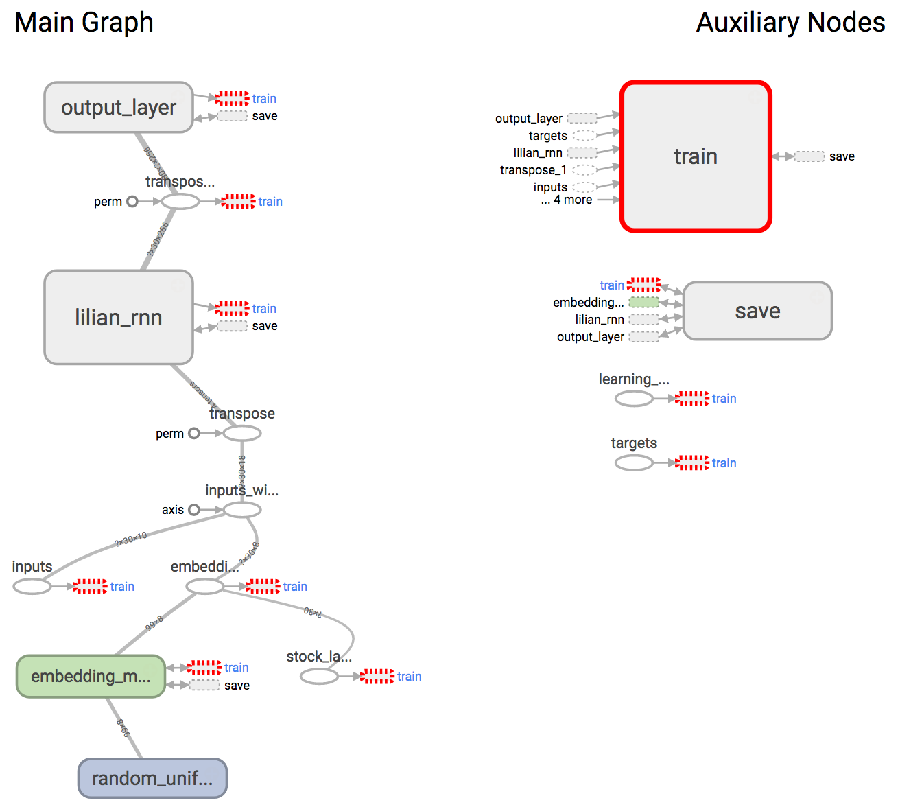
After defining the graph in code, inspect it in TensorBoard to confirm that components are constructed correctly. In practice, it closely matches the architecture diagram shown in

In addition to displaying graph structure and tracking variables over time, TensorBoard also supports embeddings visualization. To expose embedding values to TensorBoard, we must add the appropriate tracking to the training logs.

(0) For the embedding visualization, I want to color each stock by its industry sector. This metadata must be stored in a CSV file. The file contains two columns: the stock symbol and the industry sector. The CSV may or may not include a header, but the order of listed stocks must match label_encoder.classes_.

import csv
embedding_metadata_path = os.path.join(your_log_file_folder, 'metadata.csv')
with open(embedding_metadata_path, 'w') as fout:
    csv_writer = csv.writer(fout)
    # write the content into the csv file.
    # for example, csv_writer.writerows(["GOOG", "information_technology"])

(1) First, set up the summary writer within the training tf.Session.

from tensorflow.contrib.tensorboard.plugins import projector
with tf.Session(graph=lstm_graph) as sess:
    summary_writer = tf.summary.FileWriter(your_log_file_folder)
    summary_writer.add_graph(sess.graph)

(2) Add the tensor embedding_matrix, defined in our graph lstm_graph, to the projector config variable, and attach the metadata CSV file.

    projector_config = projector.ProjectorConfig()
    # You can add multiple embeddings. Here we add only one.
    added_embedding = projector_config.embeddings.add()
    added_embedding.tensor_name = embedding_matrix.name
    # Link this tensor to its metadata file.
    added_embedding.metadata_path = embedding_metadata_path

(3) This line generates a file projector_config.pbtxt in the folder your_log_file_folder. TensorBoard reads this file on startup.

    projector.visualize_embeddings(summary_writer, projector_config)

Results

The model is trained on the top 50 stocks by market value in the S&P 500 index.

(Run the following command within github.com/lilianweng/stock-rnn)

python main.py --stock_count=50 --embed_size=3 --input_size=3 --max_epoch=50 --train

The following configuration is used:

stock_count = 100
input_size = 3
embed_size = 3
num_steps = 30
lstm_size = 256
num_layers = 1
max_epoch = 50
keep_prob = 0.8
batch_size = 64
init_learning_rate = 0.05
learning_rate_decay = 0.99
init_epoch = 5

Price Prediction

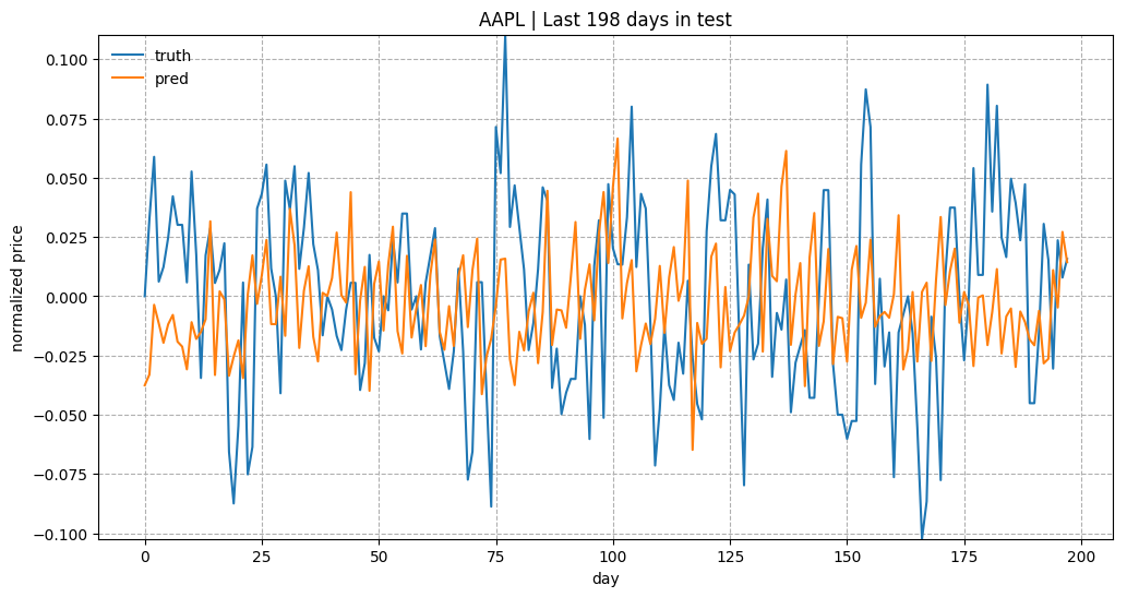
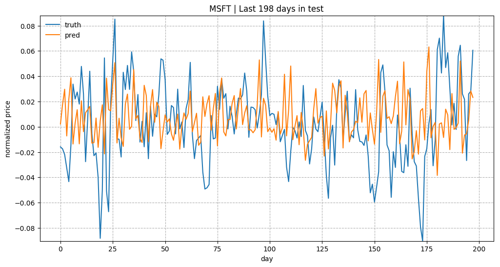
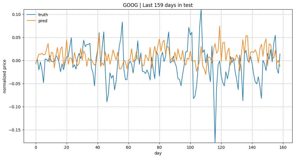
As a brief overview of prediction quality, Fig. 3 shows predictions on the test data for “KO”, “AAPL”, “GOOG”, and “NFLX”. Overall, the predicted values track the true trends well. Given how the task is set up, the model uses all historical data points to predict only the next 5 (input_size) days. With a small input_size, the model does not need to account for the long-term growth curve. Once we increase input_size, prediction becomes much more difficult.

Embedding Visualization

A standard method for visualizing clusters in embedding space is t-SNE (Maaten and Hinton, 2008), which TensorBoard supports well. t-SNE, short for “t-Distributed Stochastic Neighbor Embedding”, is a variant of Stochastic Neighbor Embedding (Hinton and Roweis, 2002) with a modified cost function that is easier to optimize.

1. As with SNE, t-SNE first converts high-dimensional Euclidean distances between points into conditional probabilities that represent similarities.
2. t-SNE defines a corresponding probability distribution in the low-dimensional space, then minimizes the Kullback–Leibler divergence between the two distributions with respect to the positions of the points in the map.

See this post for guidance on tuning t-SNE visualization parameters, including perplexity and learning rate (epsilon).

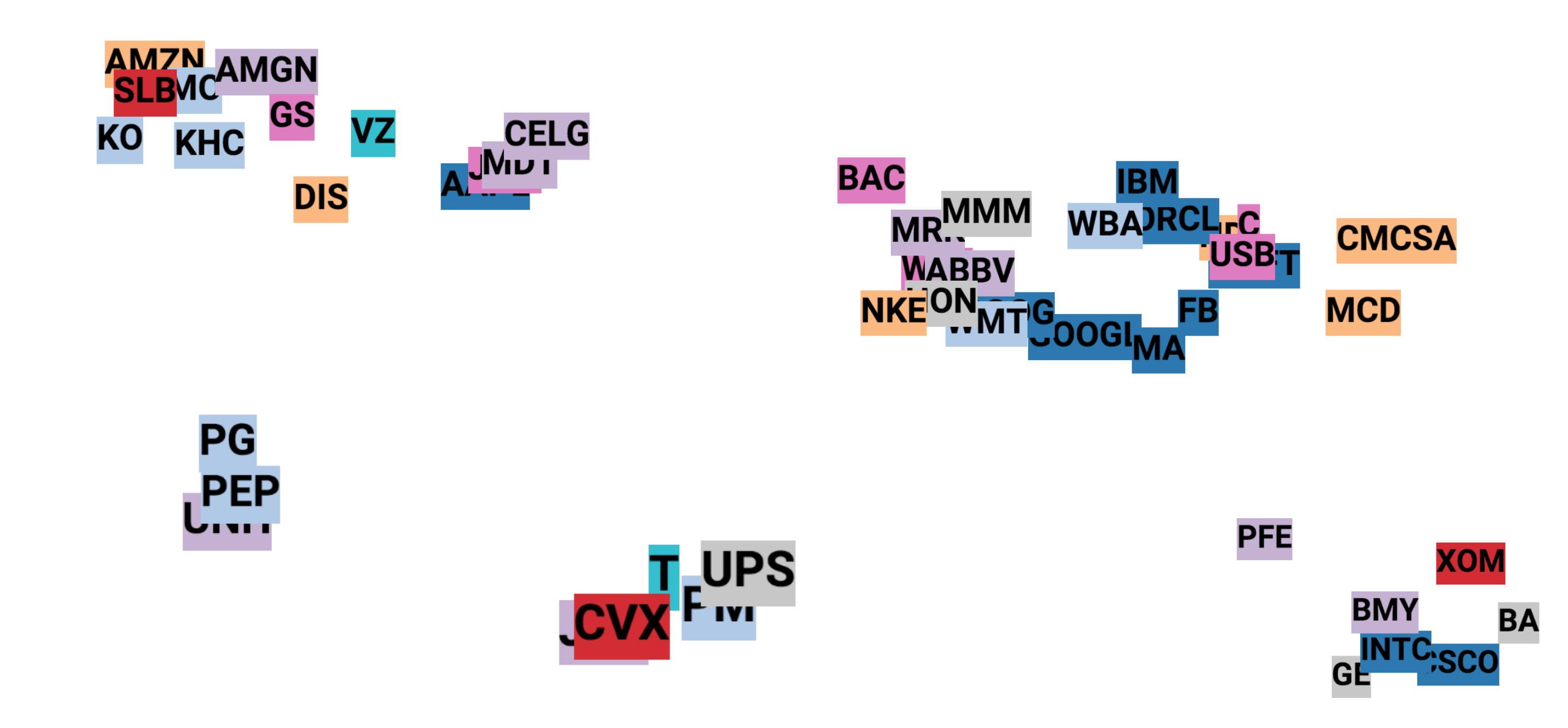
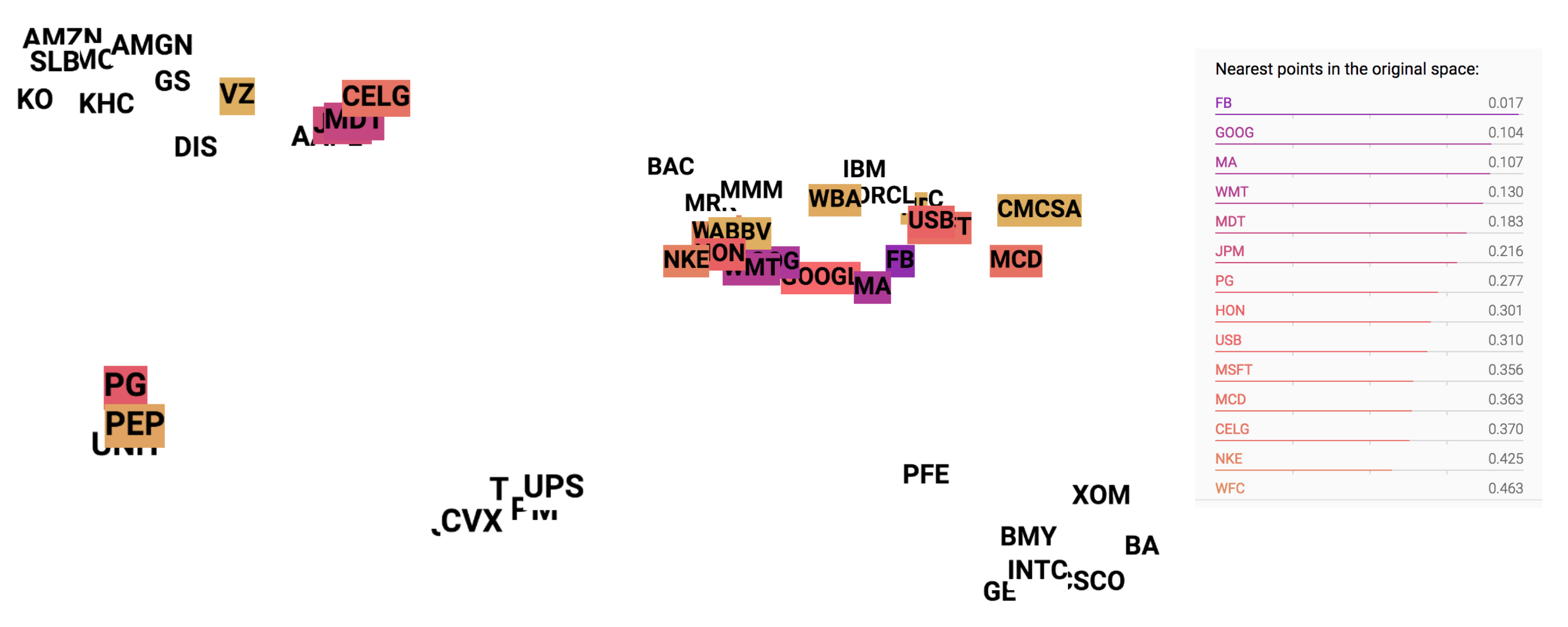
Within the embedding space, stock similarity can be evaluated by comparing their embedding vectors. For example, in the learned embeddings, GOOG is most similar to GOOGL (see Fig. 5).

Known Problems

• As training progresses, predicted values become noticeably diminished and overly flat. This is why I multiplied the absolute values by a constant to make the trend more visible in Fig. 3., since I am primarily interested in whether the model predicts the up-or-down direction correctly. Still, the diminishing prediction issue likely has a cause. Potentially, instead of using simple MSE as the loss, we could use another loss form that penalizes incorrect direction predictions more heavily.
• The loss drops quickly at the start, but it exhibits occasional value explosions (a sudden spike that then immediately returns to normal). I suspect this is also related to the loss formulation. A revised and more effective loss function may resolve the issue.

The complete code for this tutorial is available in github.com/lilianweng/stock-rnn.