Machine learning models are increasingly deployed in high-stakes domains such as health care, judicial systems, and the financial industry. As a result, it has become necessary to understand how these models reach decisions and to ensure that the decisioning process aligns with ethnic requirements or legal regulations.

At the same time, the rapid rise of deep learning further intensifies the need to interpret complex models. People want to apply the full power of AI to essential parts of everyday life, but doing so is difficult without sufficient trust in the models or an effective process for diagnosing unintended behavior, especially because deep neural networks are, by design, black boxes.

Consider the following situations:

1. The financial industry is highly regulated. Loan issuers are legally required to make fair decisions and to explain their credit models by providing reasons whenever they decline a loan application.
2. A medical diagnosis model can affect human life. How can we be sufficiently confident to treat a patient based on the recommendation of a black-box model?
3. When a criminal decision model is used in court to predict recidivism risk, we must ensure that it behaves in an equitable, honest, and nondiscriminatory manner.
4. If a self-driving car suddenly behaves abnormally and we cannot explain why, will we be comfortable deploying the technology at large scale in real traffic?

At Affirm, we issue tens of thousands of installment loans every day, and our underwriting model must provide declination reasons when it rejects an application. That is one of many motivations for me to explore this topic more deeply and write this post. Model interpretability is a broad area within machine learning. This review is not meant to cover every study, but rather to provide a starting point.

Interpretable Models

Lipton (2017) summarized key properties of an interpretable model in the theoretical review paper “The mythos of model interpretability”: a human can reproduce (“simulatability”) the computation process with a complete understanding of the algorithm (“algorithmic transparency”), and each individual component of the model admits an intuitive explanation (“decomposability”).

Many classic models have comparatively simple formulations and, as a result, come with natural, model-specific interpretation methods. In addition, new tools are being developed to support the construction of more interpretable models (Been, Khanna, & Koyejo, 2016; Lakkaraju, Bach & Leskovec, 2016).

Regression

A general form of a linear regression model is:

$ y = w_0 + w_1 x_1 + w_2 x_2 + … + w_n x_n $

The coefficients represent the change in the response associated with a one-unit increase in the independent variables. However, coefficients are not directly comparable unless features have been standardized (see sklearn.preprocessing.StandardScalar and RobustScaler), because “one unit” can mean very different things across different features. Without standardization, the product $w_i \dot x_i$ can be used to quantify a feature’s contribution to the response.

Naive Bayes

Naive Bayes is described as “naive” because it relies on a strongly simplified assumption: features are independent of one another, and each feature contributes to the output independently.

Given a feature vector $\mathbf{x} = [x_1, x_2, \dots, x_n]$ and a class label $c \in \{1, 2, \dots, C\}$, the probability that the data point belongs to that class is:

The Naive Bayes classifier is then defined as:

$ \hat{y} = \arg\max_{c \in 1, \dots, C} p(c) \prod_{i=1}^n p(x_i | c) $

Because the model learns the prior $p(x_i \vert c)$ during training, the contribution of an individual feature value can be measured directly using the posterior $p(c \vert x_i) = p(c)p(x_i \vert c) / p(x_i)$.

Decision Tree/Decision Lists

Decision lists consist of boolean functions, typically expressed using syntax such as if... then... else.... The if-condition includes a function over one or more features and yields a boolean output. Decision lists are inherently interpretable and can be visualized in a tree structure. Much of the research on decision lists is motivated by medical applications, where interpretability is often nearly as important as predictive performance.

Several types of decision lists are briefly summarized below:

• Falling Rule Lists (FRL) (Wang and Rudin, 2015) strictly enforce monotonicity over feature values. One key idea, for example in binary classification, is that the probability of prediction $Y=1$ associated with each rule decreases as one moves down the list.
• Bayesian Rule List (BRL) (Letham et al., 2015) is a generative model that produces a posterior distribution over possible decision lists.
• Interpretable Decision Sets (IDS) (Lakkaraju, Bach & Leskovec, 2016) provide a prediction framework that learns a set of classification rules. The learning objective is optimized simultaneously for accuracy and interpretability. IDS is closely related to the BETA method described later for interpreting black-box models.

Random Forests

Somewhat surprisingly, many people treat the Random Forests model as a black box, which is not accurate. A random forest produces its output via majority vote across many independent decision trees, and each individual tree is naturally interpretable.

The influence of individual features can be assessed by examining one tree at a time. Global feature importance in random forests can be quantified by the total decrease in node impurity averaged across all trees in the ensemble (the “mean decrease impurity”).

For a specific instance, because the decision paths through all trees are tracked, one can approximate the contribution of a split by taking the difference between the mean value of data points in a parent node and that in the child node. For additional details, see this blog series: Interpreting Random Forests.

Interpreting Black-Box Models

Many models are not designed with interpretability as a goal. Methods for explaining a black-box model attempt to extract information from a trained model to justify its predictions without requiring knowledge of the model’s internal mechanics. Keeping the interpretation process independent of the underlying implementation is valuable in real-world deployments: even if the base model is continuously upgraded and refined, an interpretation layer built on top does not need to be tightly coupled to those changes.

When we do not have to preserve model transparency, we can increase expressive power by adding parameters and nonlinear computation. This tradeoff helps explain why deep neural networks have been successful on tasks with rich inputs.

There is no strict requirement for how an explanation must be presented, but the central question is typically: Can I trust this model? When we rely on a model for critical or life-and-death decisions, we must establish trustworthiness in advance.

An interpretation framework typically balances two objectives:

• Fidelity: predictions produced by the explanation should match those of the original model as closely as possible.
• Interpretability: the explanation should be simple enough for humans to understand.

Side Notes: The next three methods are designed for local interpretation.

Prediction Decomposition

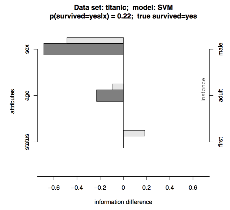
Robnik-Sikonja and Kononenko (2008) proposed explaining a single-instance prediction by measuring the difference between the original prediction and the prediction obtained after omitting a set of features.

Suppose we want to produce an explanation for a classification model $f: \mathbf{X} \rightarrow \mathbf{Y}$. Given a data point $x \in X$ that consists of $a$ attribute values $A_i$, $i = 1, \dots, a$ and is labeled as class $y \in Y$, the prediction difference is computed as the difference between predicted probabilities with and without access to $A_i$:

$ \text{probDiff}_i (y | x) = p(y| x) - p(y | x \backslash A_i) $

(The paper also discusses using the odds ratio or an entropy-based information metric to quantify prediction difference.)

Problem: If the target model already outputs probabilities, then computing $ p(y \vert x) $ is straightforward. Otherwise, the model’s prediction must be passed through a suitable post-model calibration step to translate scores into probabilities. This calibration layer introduces additional complexity.

Another problem: If we create $x \backslash A_i$ by replacing $A_i$ with a missing value (for example, None, NaN, etc.), we must rely on the model’s internal missing-value handling. A model that imputes missing values with the median can behave very differently from one that imputes a special placeholder. The paper proposes a solution: replace $A_i$ with all possible values of that feature and sum the resulting predictions weighted by the probability of observing each value in the data:

Here, $p(y \vert x \leftarrow A_i=a_s)$ is the probability of label $y$ when feature $A_i$ is set to value $a_s$ within the feature vector of $x$. There are $m_i$ distinct values of $A_i$ in the training set.

Using prediction-difference measurements obtained by omitting known features, we can decompose the contribution of each individual feature to the prediction.

Local Gradient Explanation Vector

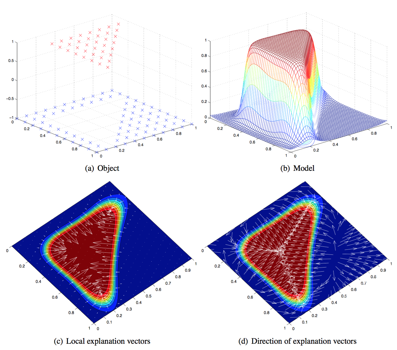
This method (Baehrens, et al. 2010) explains local decisions made by arbitrary nonlinear classification algorithms by using local gradients that describe how a data point must move in order to change its predicted label.

Assume we have a Bayes Classifier trained on dataset $X$, producing probabilities over class labels $Y$, $p(Y=y \vert X=x)$. A class label $y$ is drawn from the pool $\{1, 2, \dots, C\}$. The Bayes classifier is defined as:

$ f^{*}(x) = \arg \min_{c \in \{1, \dots, C\}} p(Y \neq c \vert X = x) $

The local explanation vector is the derivative of the probability prediction function evaluated at the test point $x = x_0$. Large entries in this vector identify features with strong influence on the model’s decision. A positive entry indicates that increasing the feature would decrease the probability of $x_0$ assigned to $f^{*}(x_0)$.

However, as with “Prediction Decomposition”, this approach requires probability outputs. If the original model (denoted $f$) is not calibrated to produce probabilities, the paper suggests approximating $f$ with another classifier that resembles the Bayes classifier $f^{*}$:

(1) Apply a Parzen window to the training data to estimate weighted class densities:

$ \hat{p}_{\sigma}(x, y=c) = \frac{1}{n} \sum_{i \in I_c} k_{\sigma} (x - x_i) $

Where $I_c$ is the index set of points assigned to class $c$ by model $f$, $I_c = \{i \vert f(x_i) = c\}$. $k_{\sigma}$ is a kernel function, and the Gaussian kernel is a common choice among many candidates.

(2) Next, apply Bayes’ rule to approximate the probabilities $p(Y=c \vert X=x)$ for all classes:

(3) The resulting estimated Bayes classifier is:

$ \hat{f}_{\sigma} = \arg\min_{c \in \{1, \dots, C\}} \hat{p}_{\sigma}(y \neq c \vert x) $

Note that labeled data can be generated from the original model $f$ in arbitrary quantity, so this procedure is not constrained by the size of the original training set. The hyperparameter $\sigma$ is chosen to maximize the likelihood that $\hat{f}_{\sigma}(x) = f(x)$ achieves high fidelity.

Side notes: As you can see both the methods above require the model prediction to be a probability. Calibration of the model output adds another layer of complication.

LIME (Local Interpretable Model-Agnostic Explanations)

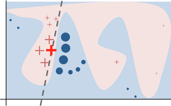
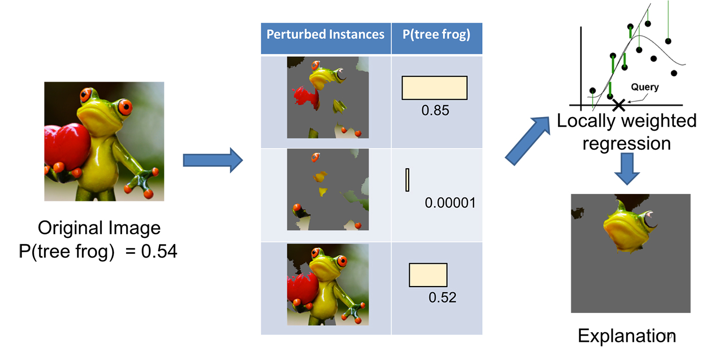
LIME, short for local interpretable model-agnostic explanation, approximates a black-box model locally in the neighborhood of the prediction of interest (Ribeiro, Singh, & Guestrin, 2016).

As above, denote the black-box model by $f$. LIME proceeds as follows:

(1) Convert the dataset into an interpretable representation: $x \Rightarrow x_b$.

• Text classifier: a binary vector indicating whether each word is present or absent.
• Image classifier: a binary vector indicating whether each contiguous region of similar pixels (a super-pixel) is present or absent.

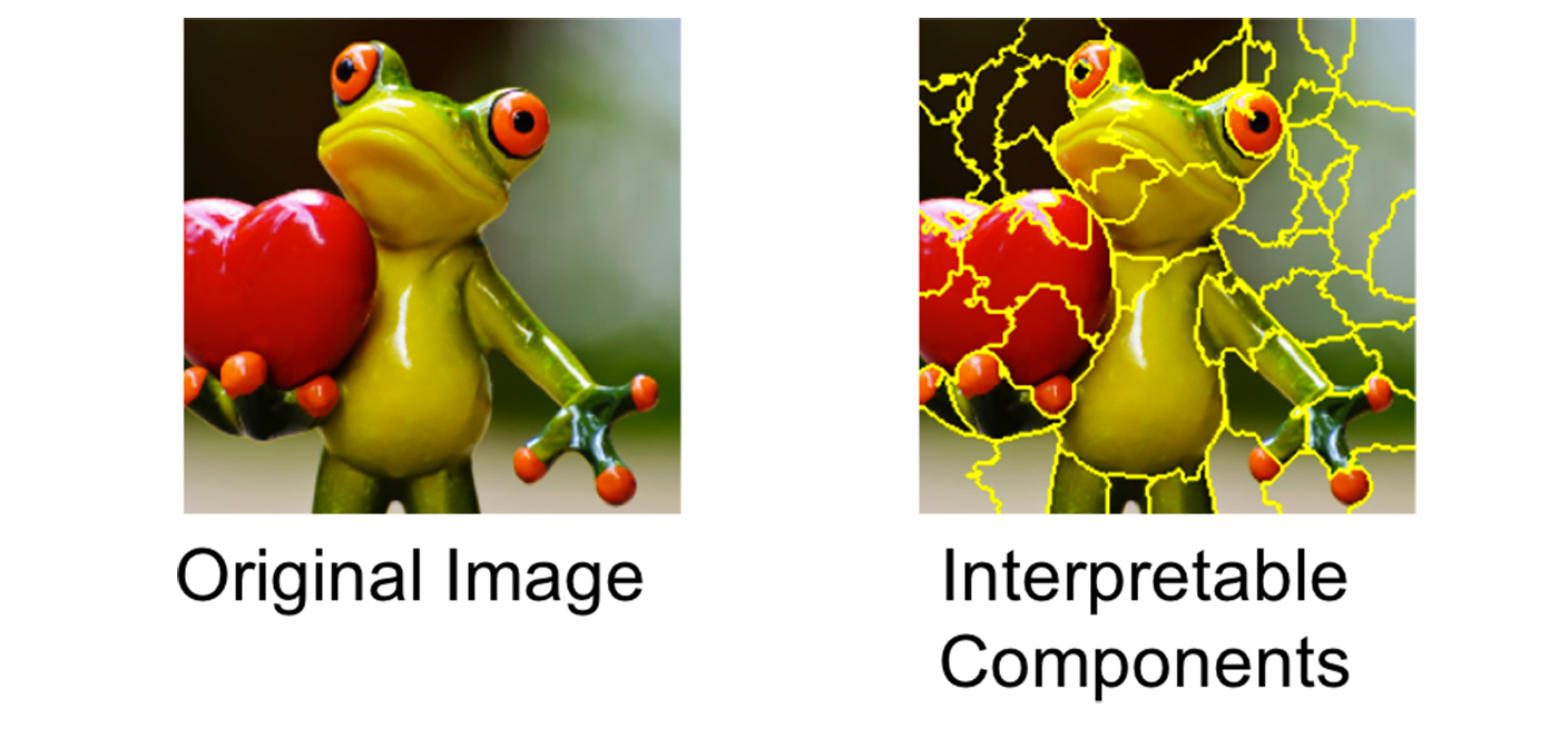
(2) Given a prediction $f(x)$ with the corresponding interpretable representation $x_b$, sample instances around $x_b$ by uniformly drawing nonzero elements of $x_b$ at random, where the number of such draws is itself uniformly sampled. This yields a perturbed sample $z_b$ that contains only a fraction of the nonzero elements of $x_b$.

Then convert $z_b$ back to the original input format $z$ and obtain a prediction score $f(z)$ from the target model.

Using many sampled points $z_b \in \mathcal{Z}_b$ and their corresponding predictions, we can fit a locally faithful explanation model (for example, a simple regression). Samples are weighted based on their proximity to $x_b$. The paper uses a lasso regression with preprocessing to select the top $k$ most significant features first, calling the procedure “K-LASSO”.

Assessing whether an explanation is reasonable can directly determine whether a model is trustworthy, because models sometimes exploit spurious correlations or generalize in unintended ways. One example in the paper applies LIME to an SVM text classifier that distinguishes “Christianity” from “Atheism”. The model achieved strong accuracy (94% on a held-out test set), but LIME showed that decisions depended on arbitrary tokens such as “re”, “posting”, and “host”, which are not directly related to either “Christianity” or “Atheism”. This diagnosis indicates that, despite good accuracy, the model should not be trusted. It also suggests concrete improvement directions, such as better text preprocessing.

For a more detailed, non-paper explanation, see this blog post by the author. A very nice read.

Side Notes: Local interpretation is generally easier than global interpretation, but harder to maintain (consider the curse of dimensionality). The methods below aim to explain overall model behavior. However, a global approach cannot capture fine-grained effects, for example when a feature is important in one region but not in another.

Feature Selection

In essence, classic feature selection methods (Yang and Pedersen, 1997; Guyon and Elisseeff, 2003) can also be viewed as global explanation techniques. Feature selection decomposes the contributions of multiple features, making it possible to explain overall model output in terms of individual feature impact.

There are many resources on feature selection, so I will skip the topic in this post.

BETA (Black Box Explanation through Transparent Approximations)

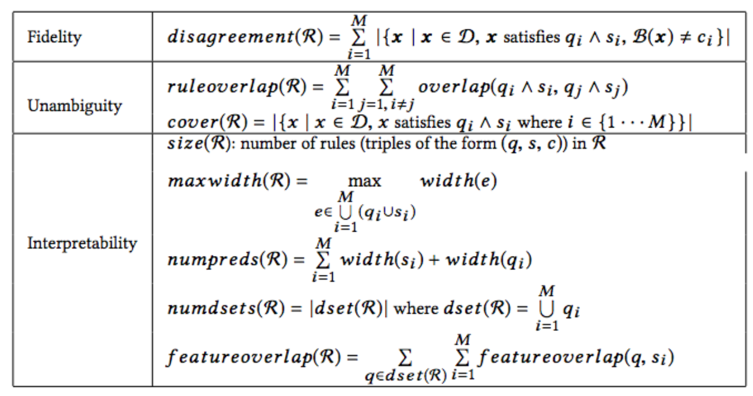
BETA, short for black box explanation through transparent approximations, is closely related to Interpretable Decision Sets (Lakkaraju, Bach & Leskovec, 2016). BETA learns a compact, two-level decision set in which each rule explains a portion of the model behavior unambiguously.

The authors proposed a novel objective function so that learning is optimized for high fidelity (strong agreement between the explanation and the model), low unambiguity (minimal overlap among decision rules in the explanation), and high interpretability (a lightweight, small explanation decision set). These aspects are combined into a single objective function to optimize.

Explainable Artificial Intelligence

This section borrows its name from the DARPA program “Explainable Artificial Intelligence”. The Explainable AI (XAI) program aims to develop more interpretable models and to enable humans to understand, appropriately trust, and effectively manage the emerging generation of artificially intelligent techniques.

As deep learning applications have advanced, concerns have grown that we may never know even if the model goes bad. The complex architecture, the large number of learnable parameters, nonlinear mathematical operations, and some intriguing properties (Szegedy et al., 2014) together contribute to the non-interpretability of deep neural networks, creating a true black box. At the same time, deep learning’s effectiveness originates in this very complexity because it provides flexibility for capturing rich and intricate patterns in real-world data.

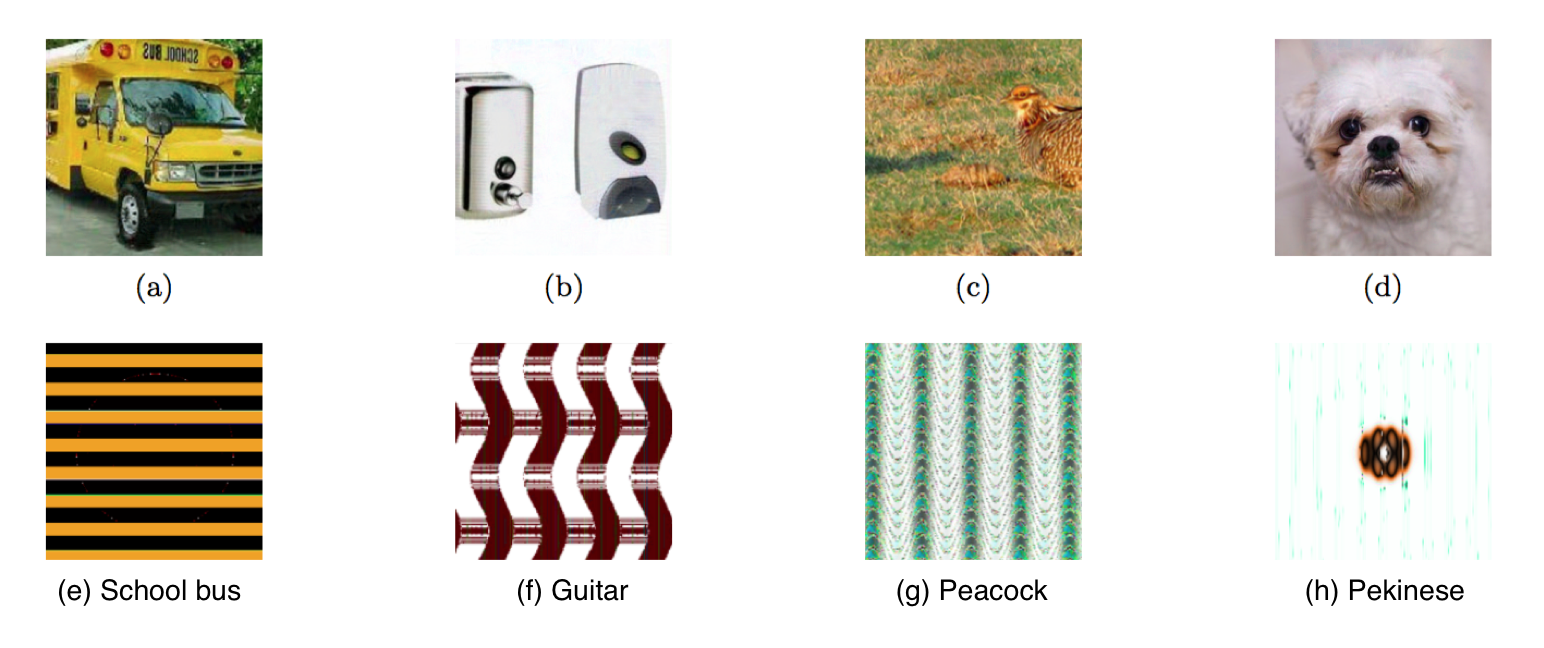
Research on adversarial examples (OpenAI Blog: Robust Adversarial Examples, Attacking Machine Learning with Adversarial Examples, Goodfellow, Shlens & Szegedy, 2015; Nguyen, Yosinski, & Clune, 2015) highlights risks to robustness and safety in AI applications. Models can exhibit unintended, unexpected, and unpredictable behavior, and we often lack a fast or effective strategy to determine why.

Nvidia recently introduced a method to visualize the pixel locations that matter most in its self-driving cars’ decision-making process. This visualization offers useful insight into how the AI “thinks” and what the system depends on while the vehicle is in operation. When the AI’s notion of what is important aligns with how humans would make comparable decisions, it can naturally increase our confidence in an otherwise black-box model.

This is a rapidly developing area, and new results and announcements appear every day. I hope this post provides a few pointers and encourages you to explore the topic further :)

Cited as:

@article{weng2017gan,
  title   = "How to Explain the Prediction of a Machine Learning Model?",
  author  = "Weng, Lilian",
  journal = "lilianweng.github.io",
  year    = "2017",
  url     = "https://lilianweng.github.io/posts/2017-08-01-interpretation/"
}

References

[1] Zachary C. Lipton. “The mythos of model interpretability.” arXiv preprint arXiv:1606.03490 (2016).

[2] Been Kim, Rajiv Khanna, and Oluwasanmi O. Koyejo. “Examples are not enough, learn to criticize! criticism for interpretability.” Advances in Neural Information Processing Systems. 2016.

[3] Himabindu Lakkaraju, Stephen H. Bach, and Jure Leskovec. “Interpretable decision sets: A joint framework for description and prediction.” Proc. 22nd ACM SIGKDD Intl. Conf. on Knowledge Discovery and Data Mining. ACM, 2016.

[4] Robnik-Šikonja, Marko, and Igor Kononenko. “Explaining classifications for individual instances.” IEEE Transactions on Knowledge and Data Engineering 20.5 (2008): 589-600.

[5] Baehrens, David, et al. “How to explain individual classification decisions.” Journal of Machine Learning Research 11.Jun (2010): 1803-1831.

[6] Marco Tulio Ribeiro, Sameer Singh, and Carlos Guestrin. “Why should I trust you?: Explaining the predictions of any classifier.” Proc. 22nd ACM SIGKDD Intl. Conf. on Knowledge Discovery and Data Mining. ACM, 2016.

[7] Yiming Yang, and Jan O. Pedersen. “A comparative study on feature selection in text categorization.” Intl. Conf. on Machine Learning. Vol. 97. 1997.

[8] Isabelle Guyon, and André Elisseeff. “An introduction to variable and feature selection.” Journal of Machine Learning Research 3.Mar (2003): 1157-1182.

[9] Ian J. Goodfellow, Jonathon Shlens, and Christian Szegedy. “Explaining and harnessing adversarial examples.” ICLR 2015.

[10] Christian Szegedy, Wojciech Zaremba, Ilya Sutskever, Joan Bruna, Dumitru Erhan, Ian Goodfellow, Rob Fergus. “Intriguing properties of neural networks.” Intl. Conf. on Learning Representations (2014)

[11] Nguyen, Anh, Jason Yosinski, and Jeff Clune. “Deep neural networks are easily fooled: High confidence predictions for unrecognizable images.” Proc. IEEE Conference on Computer Vision and Pattern Recognition. 2015.

[12] Benjamin Letham, Cynthia Rudin, Tyler H. McCormick, and David Madigan. “Interpretable classifiers using rules and Bayesian analysis: Building a better stroke prediction model.” The Annals of Applied Statistics 9, No. 3 (2015): 1350-1371.

[13] Haohan Wang, Bhiksha Raj, and Eric P. Xing. “On the Origin of Deep Learning.” arXiv preprint arXiv:1702.07800 (2017).

[14] OpenAI Blog: Robust Adversarial Examples

[15] Attacking Machine Learning with Adversarial Examples

[16] Reading an AI Car’s Mind: How NVIDIA’s Neural Net Makes Decisions