From GAN to WGAN
[Updated on 2018-09-30: thanks to Yoonju, we have this post translated in Korean!] [Updated on 2019-04-18: this post is also available on arXiv.] Generative adversarial networks (GANs) have delivered strong performance across many generative tasks that aim to reproduce rich real-world content, including images, human language, and music. The approach is motivated by game theory: two models, a generator and a critic, compete against one another, and through this competition they can simultaneously improve. Even so, training GANs is often difficult in practice, and common problems include instability during training and failures to converge.
· 21 min read · Curated and presented by Arthur Sedek
[Updated on 2018-09-30: thanks to Yoonju, we have this post translated in Korean!]
[Updated on 2019-04-18: this post is also available on arXiv.]
Generative adversarial network (GAN) has produced strong results across many generative tasks, replicating rich real-world content such as images, human language, and music. The framework is motivated by game theory: two models, a generator and a critic, compete in a way that can strengthen both over time. However, GANs can be challenging to train in practice, with common issues including training instability and failure to converge.
In the sections below, I will walk through the mathematics behind the generative adversarial network framework, explain why training can be difficult, and then introduce a modified variant of GAN intended to address these training challenges.
Kullback–Leibler and Jensen–Shannon Divergence
Before examining GANs in detail, we first review two metrics commonly used to quantify similarity between probability distributions.
(1) KL (Kullback–Leibler) divergence measures how one probability distribution $p$ diverges from a second expected probability distribution $q$.
$D_{KL}$ reaches its minimum value of zero when $p(x)$ == $q(x)$ everywhere.
From the formula, it is clear that KL divergence is asymmetric. In situations where $p(x)$ is close to zero but $q(x)$ remains significantly non-zero, the effect of $q$ is ignored. This can lead to misleading behavior when the goal is to measure similarity between two distributions that should be treated as equally important.
(2) Jensen–Shannon Divergence is another similarity measure between two probability distributions, bounded by $[0, 1]$. JS divergence is symmetric and smoother. If you would like a more detailed comparison between KL divergence and JS divergence, see this Quora post.
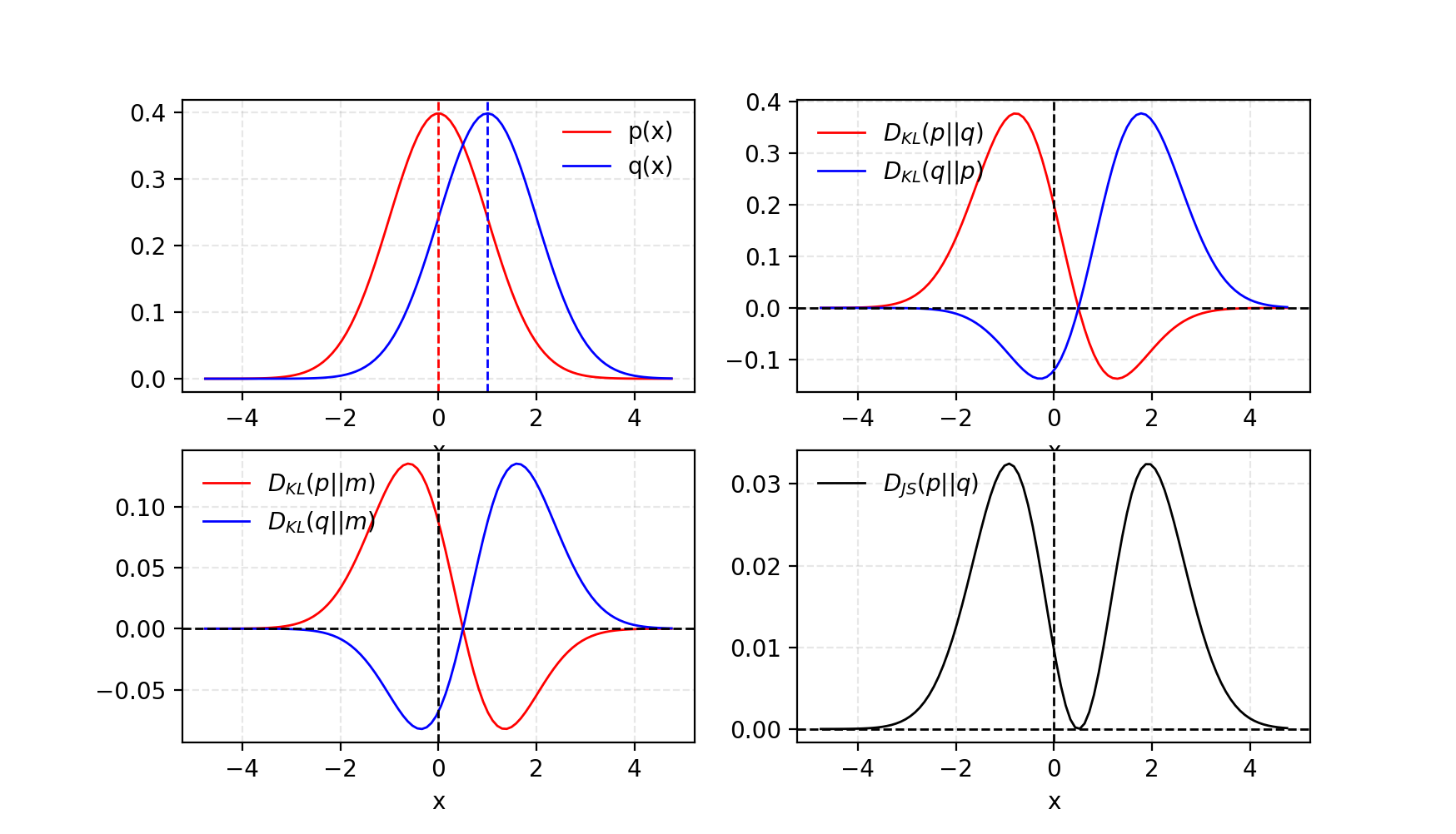
Some argue (Huszar, 2015) that one contributor to GANs’ success is the shift in the loss from the asymmetric KL divergence used in traditional maximum-likelihood approaches to the symmetric JS divergence. We will revisit this point in the next section.
Generative Adversarial Network (GAN)
A GAN is composed of two models:
- A discriminator $D$ estimates the probability that a sample comes from the real dataset. It acts as a critic and is optimized to distinguish fake samples from real ones.
- A generator $G$ produces synthetic samples given a noise variable input $z$ ($z$ introduces potential output diversity). It is trained to model the real data distribution so that generated samples appear as realistic as possible, or equivalently, so that they can fool the discriminator into assigning a high probability.
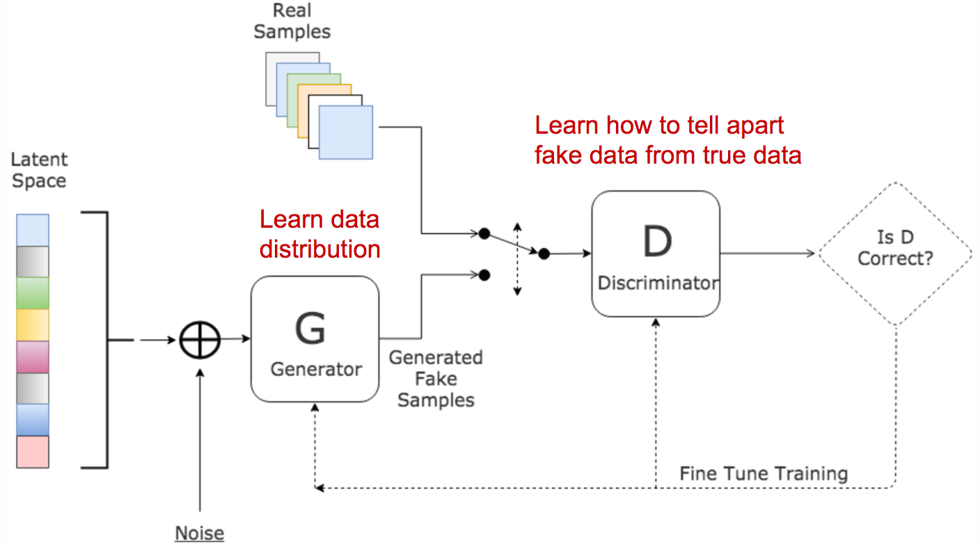
During training, these two models compete: the generator $G$ attempts to fool the discriminator, while the critic model $D$ attempts to avoid being fooled. This zero-sum game encourages both models to improve.
Given,
| Symbol | Meaning | Notes |
|---|---|---|
| $p_{z}$ | Data distribution over noise input $z$ | Usually, just uniform. |
| $p_{g}$ | The generator’s distribution over data $x$ | |
| $p_{r}$ | Data distribution over real sample $x$ |
On one side, we want the discriminator $D$ to make correct decisions on real data by maximizing $\mathbb{E}_{x \sim p_{r}(x)} [\log D(x)]$. At the same time, for a fake sample $G(z), z \sim p_z(z)$, the discriminator should output a probability $D(G(z))$ close to zero, which is achieved by maximizing $\mathbb{E}_{z \sim p_{z}(z)} [\log (1 - D(G(z)))]$.
On the other side, the generator is trained to increase the likelihood that $D$ assigns a high probability to a fake example, and thus to minimize $\mathbb{E}_{z \sim p_{z}(z)} [\log (1 - D(G(z)))]$.
Combining both objectives, $D$ and $G$ play a minimax game. The loss to optimize is:
($\mathbb{E}_{x \sim p_{r}(x)} [\log D(x)]$ does not affect $G$ during gradient descent updates.)
What is the optimal value for D?
With a well-defined objective, we first ask what value of $D$ is optimal.
Because we want the best value of $D(x)$ that maximizes $L(G, D)$, let us define:
The quantity inside the integral (and we can ignore the integral since $x$ is sampled over all possible values) is:
Therefore, setting $\frac{d f(\tilde{x})}{d \tilde{x}} = 0$ yields the optimal discriminator: $D^*(x) = \tilde{x}^* = \frac{A}{A + B} = \frac{p_{r}(x)}{p_{r}(x) + p_g(x)} \in [0, 1]$.
Once the generator reaches its optimum, $p_g$ becomes very close to $p_{r}$. When $p_g = p_{r}$, $D^*(x)$ becomes $1/2$.
What is the global optimal?
When both $G$ and $D$ attain their optimal values, we have $p_g = p_{r}$ and $D^*(x) = 1/2$, and the loss reduces to:
What does the loss function represent?
Using the formula given in the previous section, the JS divergence between $p_{r}$ and $p_g$ is:
Thus,
In other words, when the discriminator is optimal, the GAN loss measures similarity between the generated data distribution $p_g$ and the real data distribution $p_{r}$ via JS divergence. The best $G^*$, which matches the real data distribution, corresponds to the minimum $L(G^*, D^*) = -2\log2$, consistent with the equations above.
Other Variations of GAN: There are many GAN variants, either adapted to different contexts or designed for specific tasks. For semi-supervised learning, for example, one approach modifies the discriminator to output real class labels, $1, \dots, K-1$, along with one additional fake class label $K$. The generator then aims to fool the discriminator into producing a classification label smaller than $K$.
Tensorflow Implementation: carpedm20/DCGAN-tensorflow
Problems in GANs
Although GANs have demonstrated strong performance in realistic image generation, training is difficult. The process is widely recognized as slow and unstable.
Hard to achieve Nash equilibrium
Salimans et al. (2016) discussed issues with GAN training procedures based on gradient descent. The two models are trained simultaneously to find a Nash equilibrium in a two-player non-cooperative game. However, each model updates its own cost independently, without accounting for the other player. As a result, updating both gradients concurrently does not guarantee convergence.
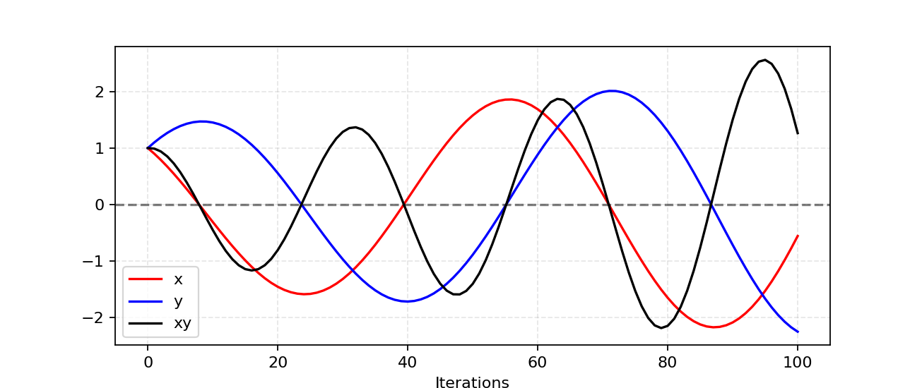
Consider a simple example to illustrate why finding a Nash equilibrium in a non-cooperative game can be difficult. Assume one player controls $x$ to minimize $f_1(x) = xy$, while the other player simultaneously updates $y$ to minimize $f_2(y) = -xy$.
Because $\frac{\partial f_1}{\partial x} = y$ and $\frac{\partial f_2}{\partial y} = -x$, we update $x$ with $x-\eta \cdot y$ and $y$ with $y+ \eta \cdot x$ simultaneously in one iteration, where $\eta$ is the learning rate. Once $x$ and $y$ have different signs, subsequent gradient updates produce large oscillations, and the instability worsens over time, as shown in
Low dimensional supports
| Term | Explanation |
|---|---|
| Manifold | A topological space that locally resembles Euclidean space near each point. Precisely, when this Euclidean space is of dimension $n$, the manifold is referred as $n$-manifold. |
| Support | A real-valued function $f$ is the subset of the domain containing those elements which are not mapped to zero. |
Arjovsky and Bottou (2017) analyzed how the supports of $p_r$ and $p_g$ often lie on low-dimensional manifolds, and how this contributes to GAN training instability, in the theoretical paper “Towards principled methods for training generative adversarial networks”.
The dimensions of many real-world datasets, represented by $p_r$, often appear artificially high. Empirically, they tend to concentrate on a lower-dimensional manifold, which is the foundational assumption behind Manifold Learning. For real-world images, once the theme or the object is fixed, the images must obey many constraints, for example, a dog should have two ears and a tail, and a skyscraper should have a straight and tall body. Such constraints keep images away from the possibility of unrestricted high-dimensional variation.
$p_g$ also lies on a low-dimensional manifold. Whenever the generator is tasked with producing a much larger image, such as 64x64, from a low-dimensional noise input such as 100, $z$, the color distribution across the 4096 pixels is determined by that 100-dimensional random vector and therefore can rarely cover the full high-dimensional space.
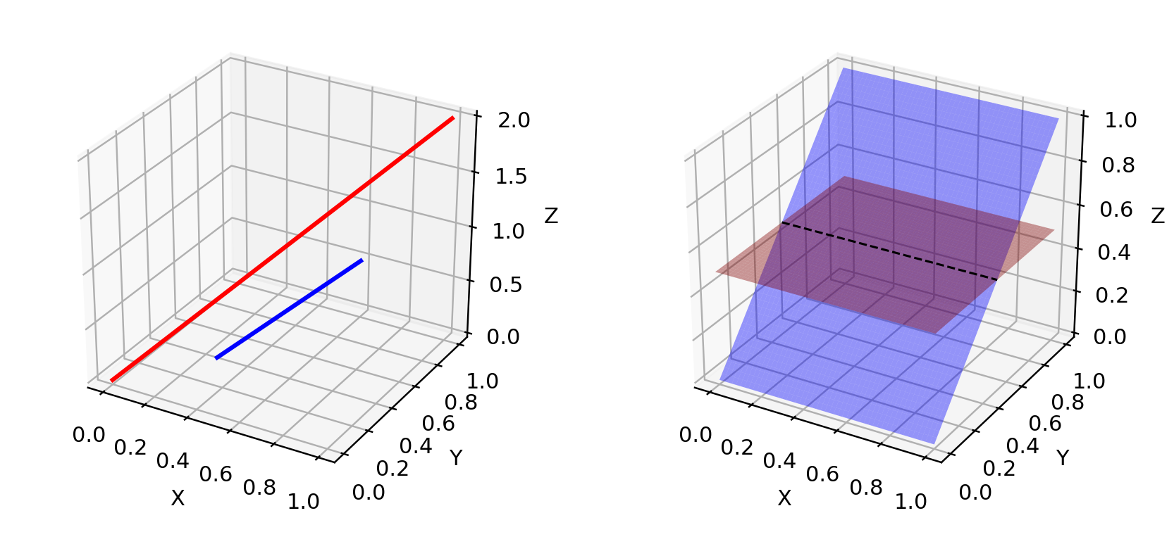
Because both $p_g$ and $p_r$ lie on low-dimensional manifolds, they are almost certainly disjoint (see Fig. 4). When their supports are disjoint, we can always find a perfect discriminator that separates real and fake samples with 100% accuracy. See the paper if you want the proof.
Vanishing gradient
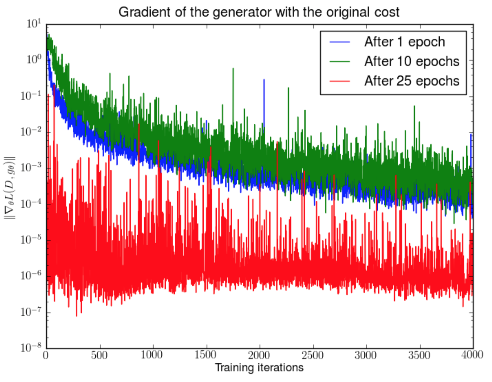
When the discriminator is perfect, we are guaranteed $D(x) = 1, \forall x \in p_r$ and $D(x) = 0, \forall x \in p_g$. Consequently, the loss $L$ drops to zero, leaving no gradient for updates during training iterations. Fig. 5 shows an experiment in which the gradient vanishes quickly as the discriminator improves.
As a result, GAN training faces a dilemma:
- If the discriminator performs poorly, the generator receives inaccurate feedback, and the loss function does not reflect reality.
- If the discriminator performs very well, the loss gradient becomes close to zero, and learning becomes extremely slow or can even stall.
This dilemma can make GAN training particularly difficult.
Mode collapse
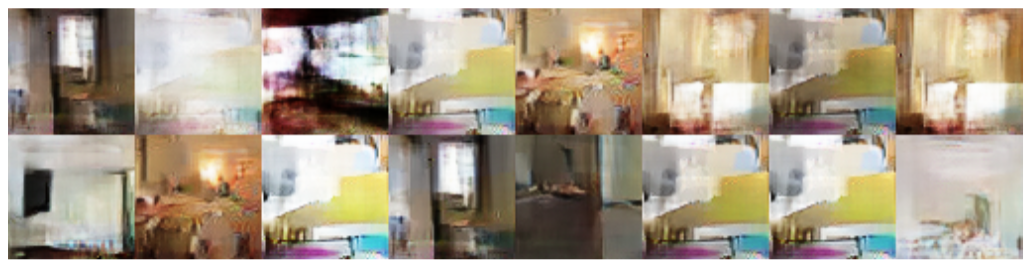
During training, the generator can collapse to a configuration in which it produces the same outputs repeatedly. This common failure mode is known as Mode Collapse. Even if the generator can fool the corresponding discriminator, it fails to learn the complexity of the real-world data distribution and becomes stuck in a small region with extremely limited variety.
Lack of a proper evaluation metric
Generative adversarial networks do not inherently provide a good objective function for monitoring training progress. Without a reliable evaluation metric, training becomes analogous to working in the dark: there is no clear signal for when to stop, and no strong indicator for comparing multiple models.
Improved GAN Training
The following suggestions have been proposed to stabilize GAN training and improve performance.
The first five methods are practical techniques to promote faster convergence, proposed in “Improve Techniques for Training GANs”. The last two are proposed in “Towards principled methods for training generative adversarial networks” to address the issue of disjoint distributions.
(1) Feature Matching
Feature matching proposes optimizing the discriminator to check whether the generator output matches the expected statistics of real samples. Under this approach, the new loss function is $| \mathbb{E}_{x \sim p_r} f(x) - \mathbb{E}_{z \sim p_z(z)}f(G(z)) |_2^2 $, where $f(x)$ can be any feature-statistics computation, such as mean or median.
(2) Minibatch Discrimination
With minibatch discrimination, the discriminator can capture relationships among training points within a batch, rather than treating each point independently.
Within a minibatch, we approximate the closeness between each pair of samples, $c(x_i, x_j)$, and summarize each data point by summing how close it is to other samples in the same batch, $o(x_i) = \sum_{j} c(x_i, x_j)$. Then $o(x_i)$ is explicitly appended to the model input.
(3) Historical Averaging
For both models, add $ | \Theta - \frac{1}{t} \sum_{i=1}^t \Theta_i |^2 $ to the loss, where $\Theta$ is the model parameter and $\Theta_i$ represents the parameter value at a past training time $i$. This additional term penalizes training when $\Theta$ changes too dramatically over time.
(4) One-sided Label Smoothing
When feeding the discriminator, replace hard labels 1 and 0 with softened values such as 0.9 and 0.1. This has been shown to reduce network vulnerability.
(5) Virtual Batch Normalization (VBN)
Each sample is normalized using a fixed batch (a “reference batch”) rather than its current minibatch. The reference batch is selected once at the beginning and remains unchanged throughout training.
Theano Implementation: openai/improved-gan
(6) Adding Noises.
Based on the discussion in the previous section, $p_r$ and $p_g$ are disjoint in a high-dimensional space, which leads to vanishing gradients. To artificially “spread out” the distributions and increase the likelihood that the two distributions overlap, one approach is to add continuous noise to the discriminator inputs $D$.
(7) Use Better Metric of Distribution Similarity
The vanilla GAN loss measures the JS divergence between the distributions of $p_r$ and $p_g$. This metric does not provide a meaningful value when the two distributions are disjoint.
Wasserstein metric is proposed as a replacement for JS divergence because it provides a much smoother value space. The next section discusses this in more detail.
Wasserstein GAN (WGAN)
What is Wasserstein distance?
Wasserstein Distance measures the distance between two probability distributions. It is also known as the Earth Mover’s distance (EM distance), because it can be interpreted (informally) as the minimum energy required to move and reshape a pile of dirt whose shape corresponds to one probability distribution into the shape of the other distribution. The cost is quantified as: the amount of dirt moved x the distance it is moved.
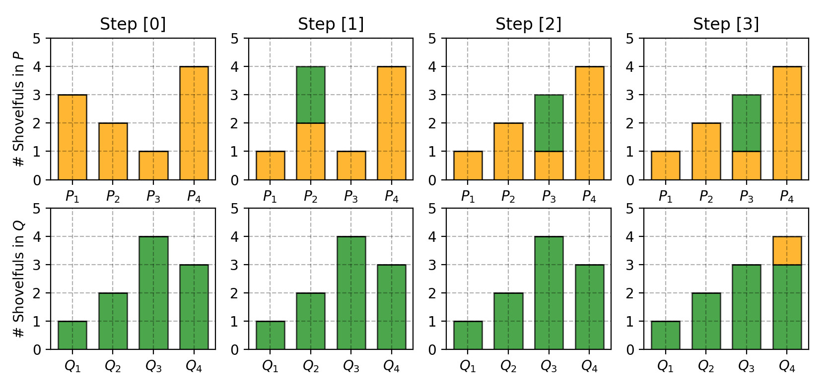
https://en.wikipedia.org/wiki/Hungarian_algorithm https://en.wikipedia.org/wiki/Transportation_theory_(mathematics)We begin with a simple discrete case. Suppose we have two distributions $P$ and $Q$. Each distribution consists of four piles of dirt, and both contain ten shovelfuls of dirt in total. The number of shovelfuls in each pile is:
To transform $P$ into $Q$, as shown in Fig. 7, we do the following:
- First move 2 shovelfuls from $P_1$ to $P_2$ => $(P_1, Q_1)$ match up.
- Then move 2 shovelfuls from $P_2$ to $P_3$ => $(P_2, Q_2)$ match up.
- Finally move 1 shovelfuls from $Q_3$ to $Q_4$ => $(P_3, Q_3)$ and $(P_4, Q_4)$ match up.
If we denote the cost required to make $P_i$ and $Q_i$ match as $\delta_i$, then $\delta_{i+1} = \delta_i + P_i - Q_i$, and for this example:
Finally, the Earth Mover’s distance is $W = \sum \vert \delta_i \vert = 5$.
For continuous probability domains, the distance is defined as:
In the expression above, $\Pi(p_r, p_g)$ is the set of all possible joint probability distributions between $p_r$ and $p_g$. A particular joint distribution $\gamma \in \Pi(p_r, p_g)$ represents one transport plan, analogous to the discrete example, but defined over a continuous probability space. Specifically, $\gamma(x, y)$ specifies what fraction of dirt should be transported from point $x$ to point $y$ so that $x$ follows the same probability distribution as $y$. This is why the marginal distribution over $x$ sums to $p_g$, $\sum_{x} \gamma(x, y) = p_g(y)$ (Once we finish moving the planned amount of dirt from every possible $x$ to the target $y$, we end up with exactly what $y$ has according to $p_g$.) and, similarly, $\sum_{y} \gamma(x, y) = p_r(x)$.
If $x$ is the origin and $y$ is the destination, then the amount of dirt moved is $\gamma(x, y)$ and the travel distance is $| x-y |$, so the cost is $\gamma(x, y) \cdot | x-y |$. The expected cost, averaged over all $(x,y)$ pairs, can be computed as:
Finally, the EM distance is defined as the minimum cost among all possible transport plans. In the definition of Wasserstein distance, $\inf$ (infimum, also known as greatest lower bound) indicates that we are concerned only with the smallest achievable cost.
Why Wasserstein is better than JS or KL divergence?
Even when two distributions lie on low-dimensional manifolds and do not overlap, Wasserstein distance can still provide a meaningful and smooth representation of the distance between them.
The WGAN paper illustrates this with a simple example.
Suppose we have two probability distributions, $P$ and $Q$:
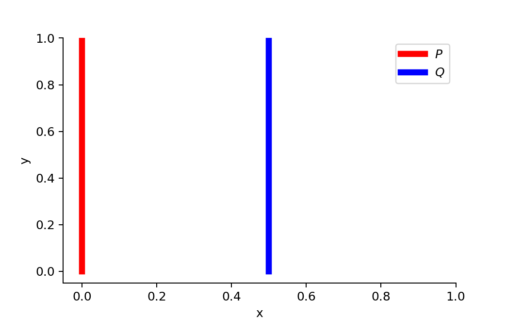
When $\theta \neq 0$:
But when $\theta = 0$, two distributions are fully overlapped:
$D_{KL}$ yields inifity when two distributions are disjoint. The value of $D_{JS}$ exhibits a sudden jump and is not differentiable at $\theta = 0$. In contrast, only the Wasserstein metric provides a smooth measure, which is highly beneficial for stable learning with gradient descents.
Use Wasserstein distance as GAN loss function
In practice, it is intractable to enumerate all possible joint distributions in $\Pi(p_r, p_g)$ in order to compute $\inf_{\gamma \sim \Pi(p_r, p_g)}$. For this reason, the authors proposed a convenient reformulation using the Kantorovich-Rubinstein duality:
Here, $\sup$ (supremum) is the counterpart of $inf$ (infimum). In this context, we seek the least upper bound, or more plainly, the maximum value.
Lipschitz continuity?
In the dual form of the Wasserstein metric, the function $f$ is required to satisfy $| f |_L \leq K$, that is, it must be K-Lipschitz continuous.
A real-valued function $f: \mathbb{R} \rightarrow \mathbb{R}$ is called $K$-Lipschitz continuous if there exists a real constant $K \geq 0$ such that, for all $x_1, x_2 \in \mathbb{R}$,
$ \lvert f(x_1) - f(x_2) \rvert \leq K \lvert x_1 - x_2 \rvert $
In this definition, $K$ is referred to as a Lipschitz constant for the function $f(.)$. Any function that is continuously differentiable everywhere is Lipschitz continuous because its derivative, estimated as $\frac{\lvert f(x_1) - f(x_2) \rvert}{\lvert x_1 - x_2 \rvert}$, is bounded. However, a Lipschitz continuous function does not need to be differentiable everywhere, as in the case of $f(x) = \lvert x \rvert$.
A full explanation of how this transformation arises from the Wasserstein distance definition would require a dedicated post, so the details are omitted here. If you want to learn how to compute the Wasserstein metric via linear programming, or how to derive the dual form via the Kantorovich-Rubinstein Duality, see this awesome post.
Assume the function $f$ is drawn from a family of K-Lipschitz continuous functions, $\{ f_w \}_{w \in W}$, parameterized by $w$. In the modified Wasserstein-GAN formulation, the “discriminator” is trained to learn $w$ by identifying a suitable $f_w$. The loss is then defined to measure the Wasserstein distance between $p_r$ and $p_g$.
Consequently, the “discriminator” is no longer a direct classifier whose role is to separate fake samples from real ones. Instead, it is trained to learn a $K$-Lipschitz continuous function that supports estimation of the Wasserstein distance. As training reduces this loss, the Wasserstein distance shrinks, and the generator’s output distribution moves closer to the real data distribution.
A key practical challenge is preserving the $K$-Lipschitz continuity of $f_w$ throughout training so that the method remains valid. The paper introduces a simple, effective heuristic: after each gradient update, clamp the weights $w$ to a narrow interval such as $[-0.01, 0.01]$. This yields a compact parameter space $W$, so $f_w$ acquires lower and upper bounds, helping maintain Lipschitz continuity.
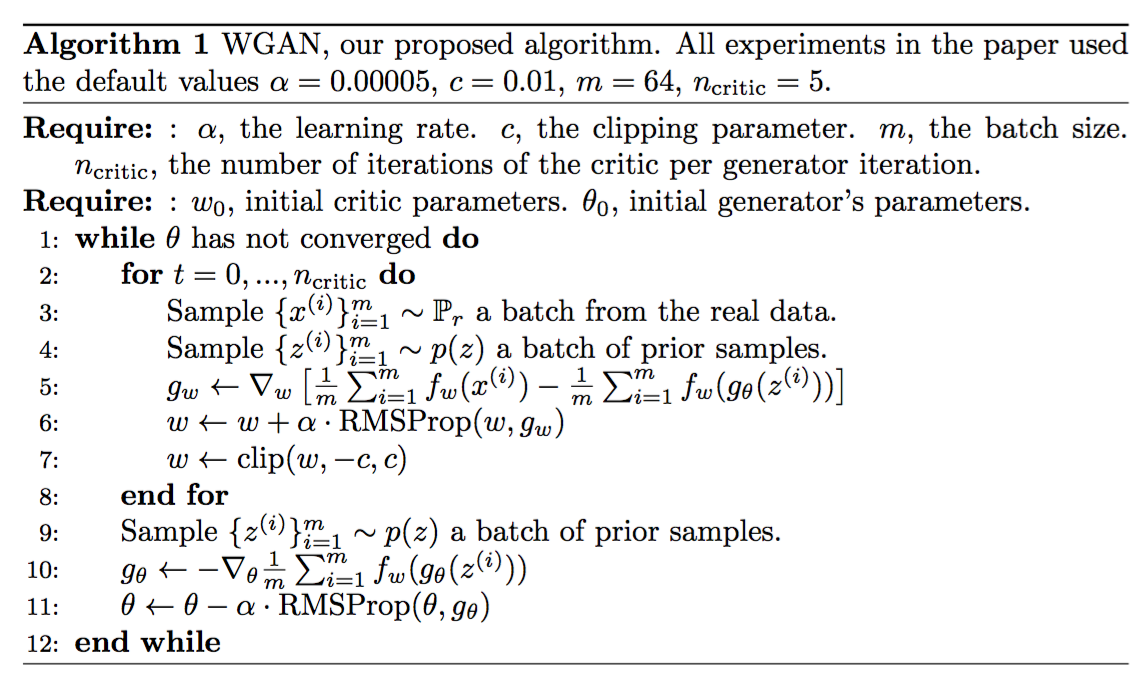
Relative to the original GAN procedure, WGAN makes the following adjustments:
- After each gradient update to the critic function, clamp the weights to a small fixed range, $[-c, c]$.
- Adopt a new loss derived from the Wasserstein distance, with no logarithm term. The “discriminator” is not used as a direct critic; instead, it serves as a tool for estimating the Wasserstein metric between the real and generated data distributions.
- Based on empirical results, the authors recommend the RMSProp optimizer for the critic, rather than a momentum-based optimizer such as Adam, which may introduce instability during training. I have not found a clear theoretical explanation for this point, though.
Unfortunately, Wasserstein GAN is not a complete solution. Even the original WGAN authors acknowledged that “Weight clipping is a clearly terrible way to enforce a Lipschitz constraint” (Oops!). In practice, WGAN can still exhibit unstable training, slow convergence after weight clipping (when the clipping window is too large), and vanishing gradients (when the clipping window is too small).
An improvement, specifically replacing weight clipping with gradient penalty, is discussed in Gulrajani et al. 2017. I will defer that topic to a future post.
Example: Create New Pokemons!
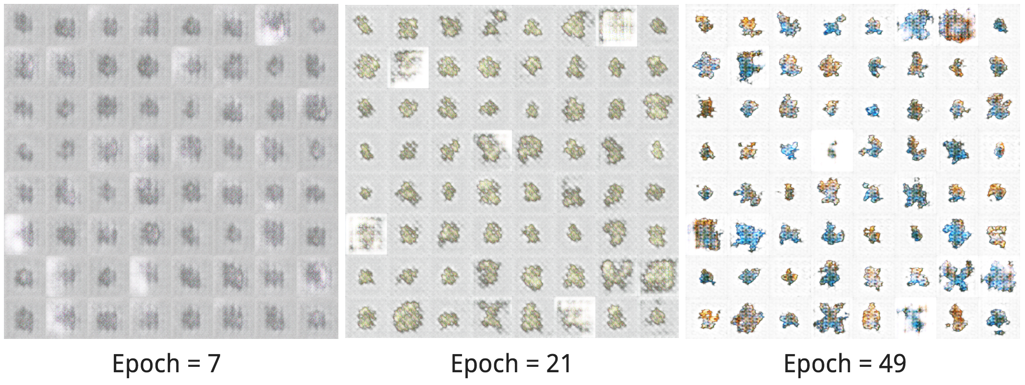
For fun, I experimented with carpedm20/DCGAN-tensorflow on a small dataset, Pokemon sprites. This dataset contains about 900 pokemon images, including multiple variants for the same pokemon species.
Let’s see what kinds of new pokemons the model can generate. Unfortunately, because the training set is so small, the samples largely capture coarse shapes with limited detail. With more training epoches, the shapes and colors do improve. Hooray!
If you would like a commented version of carpedm20/DCGAN-tensorflow, along with guidance on modifying it to train WGAN and WGAN with gradient penalty, see lilianweng/unified-gan-tensorflow.
Cited as:
@article{weng2017gan,
  title   = "From GAN to WGAN",
  author  = "Weng, Lilian",
  journal = "lilianweng.github.io",
  year    = "2017",
  url     = "https://lilianweng.github.io/posts/2017-08-20-gan/"
}
OR
@misc{weng2019gan,
    title={From GAN to WGAN},
    author={Lilian Weng},
    year={2019},
    eprint={1904.08994},
    archivePrefix={arXiv},
    primaryClass={cs.LG}
}
References
[1] Goodfellow, Ian, et al. “Generative adversarial nets.” NIPS, 2014.
[2] Tim Salimans, et al. “Improved techniques for training gans.” NIPS 2016.
[3] Martin Arjovsky and Léon Bottou. “Towards principled methods for training generative adversarial networks.” arXiv preprint arXiv:1701.04862 (2017).
[4] Martin Arjovsky, Soumith Chintala, and Léon Bottou. “Wasserstein GAN.” arXiv preprint arXiv:1701.07875 (2017).
[5] Ishaan Gulrajani, Faruk Ahmed, Martin Arjovsky, Vincent Dumoulin, Aaron Courville. Improved training of wasserstein gans. arXiv preprint arXiv:1704.00028 (2017).
[6] Computing the Earth Mover’s Distance under Transformations
[7] Wasserstein GAN and the Kantorovich-Rubinstein Duality
[8] zhuanlan.zhihu.com/p/25071913
[9] Ferenc Huszár. “How (not) to Train your Generative Model: Scheduled Sampling, Likelihood, Adversary?.” arXiv preprint arXiv:1511.05101 (2015).