Flow-based Deep Generative Models
To date, I have discussed two categories of generative models, GANs and VAEs. Neither model class learns the real data probability density function explicitly, $p(\mathbf{x})$ (where $\mathbf{x} \in \mathcal{D}$), because doing so is extremely difficult. For example, in a generative model that uses latent variables, $p(\mathbf{x}) = \int p(\mathbf{x}\vert\mathbf{z})p(\mathbf{z})d\mathbf{z}$ is very difficult to compute, since it is intractable to enumerate all possible values of the latent code $\mathbf{z}$.
· 21 min read · Curated and presented by Arthur Sedek
So far, I have written about two types of generative models, GAN and VAE. Neither of them explicitly learns the probability density function of real data, $p(\mathbf{x})$ (where $\mathbf{x} \in \mathcal{D}$), because it is extremely difficult. Using a generative model with latent variables as an example, $p(\mathbf{x}) = \int p(\mathbf{x}\vert\mathbf{z})p(\mathbf{z})d\mathbf{z}$ can hardly be computed, as it is intractable to enumerate all possible values of the latent code $\mathbf{z}$.
Flow-based deep generative models address this difficult problem with the help of normalizing flows, a powerful statistical tool for density estimation. A good estimate of $p(\mathbf{x})$ makes it possible to efficiently solve many downstream tasks: sample unobserved but realistic new data points (data generation), predict the rarity of future events (density estimation), infer latent variables, fill in incomplete data samples, and so on.
Types of Generative Models
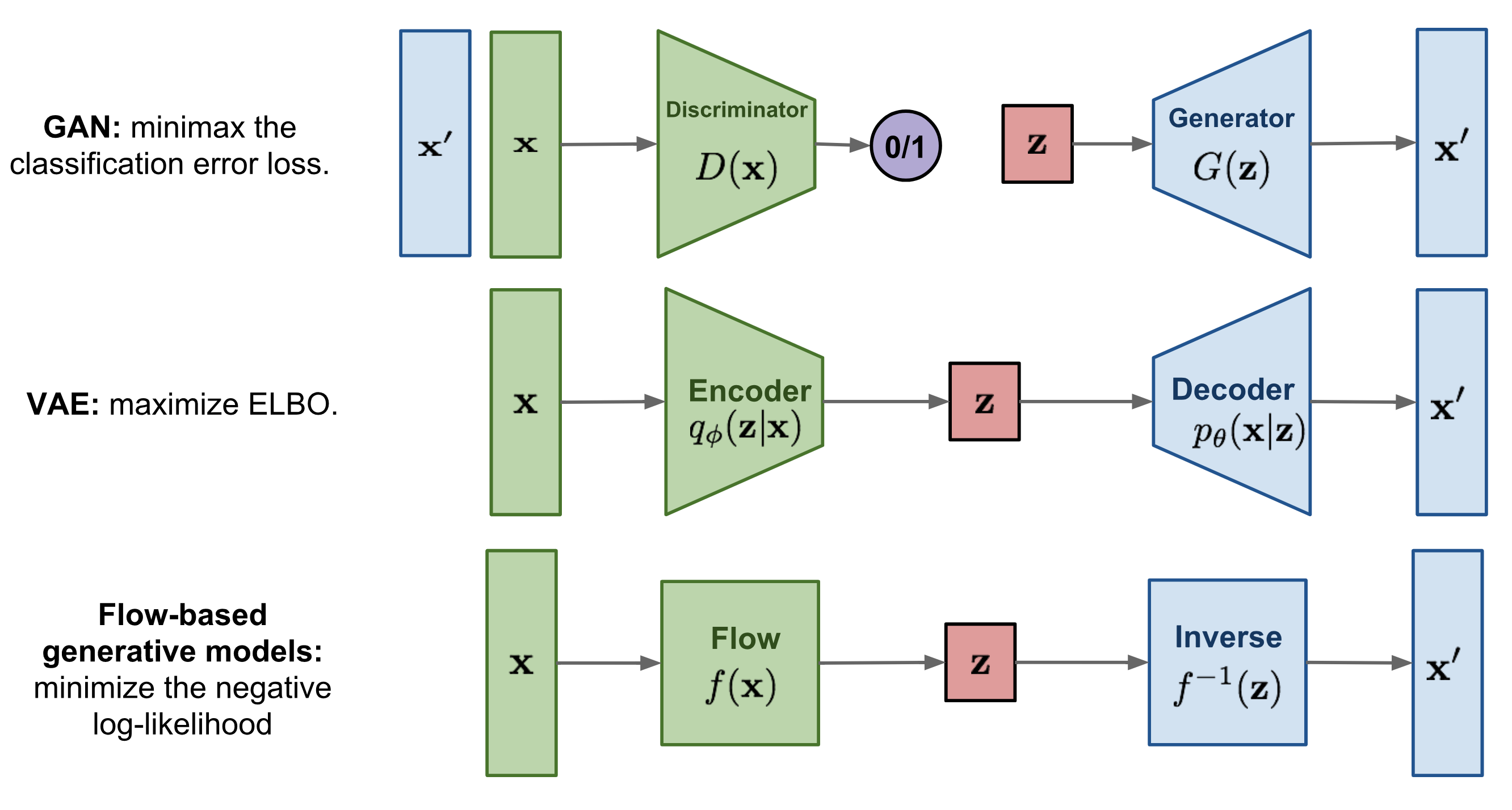
Here is a quick summary of the differences among GANs, VAEs, and flow-based generative models:
- Generative adversarial networks: GAN provides an elegant solution by framing data generation, an unsupervised learning problem, as a supervised one. The discriminator learns to distinguish real data from fake samples produced by the generator. The two models are trained as they play a minimax game.
- Variational autoencoders: VAEs implicitly optimize the data log-likelihood by maximizing the evidence lower bound (ELBO).
- Flow-based generative models: A flow-based generative model is constructed from a sequence of invertible transformations. Unlike the other two, it explicitly learns the data distribution $p(\mathbf{x})$, and therefore the loss function is simply the negative log-likelihood.
Linear Algebra Basics Recap
Before getting into flow-based generative models, we should understand two key concepts: the Jacobian determinant and the change-of-variables rule. This is fairly basic, so feel free to skip it.
Jacobian Matrix and Determinant
Given a function that maps an $n$-dimensional input vector $\mathbf{x}$ to an $m$-dimensional output vector, $\mathbf{f}: \mathbb{R}^n \mapsto \mathbb{R}^m$, the matrix of all first-order partial derivatives of this function is called the Jacobian matrix, $\mathbf{J}$, where the entry in the $i$-th row and $j$-th column is $\mathbf{J}_{ij} = \frac{\partial f_i}{\partial x_j}$.
The determinant is a real number computed as a function of all the elements in a square matrix. Note that the determinant only exists for square matrices. The absolute value of the determinant can be thought of as a measure of “how much multiplication by the matrix expands or contracts space”.
The determinant of an $n \times n$ matrix $M$ is:
where the subscripts under the summation $j_1 j_2 \dots j_n$ are all permutations of the set {1, 2, …, n}, so there are $n!$ items in total; $\tau(.)$ indicates the signature sign
of a permutation.singular matrix with linearly dependent rows or columns; or any row or column is all 0); otherwise, if $\det(M)\neq 0$, $M$ is invertible.
The determinant of a product equals the product of the determinants: $\det(AB) = \det(A)\det(B)$. (proof)
Change of Variable Theorem
Let’s review the change-of-variables theorem specifically in the context of probability density estimation, starting with the single-variable case.
Given a random variable $z$ with a known probability density function, $z \sim \pi(z)$, we would like to construct a new random variable using a one-to-one mapping function $x = f(z)$. The function $f$ is invertible, so $z=f^{-1}(x)$. Now the question is how to infer the unknown probability density function of the new variable, $p(x)$?
By definition, the integral $\int \pi(z)dz$ is the sum of an infinite number of rectangles of infinitesimal width $\Delta z$. The height of such a rectangle at position $z$ is the value of the density function $\pi(z)$. When we substitute variables, $z = f^{-1}(x)$ yields $\frac{\Delta z}{\Delta x} = (f^{-1}(x))’$ and $\Delta z = (f^{-1}(x))’ \Delta x$. Here $\vert(f^{-1}(x))’\vert$ indicates the ratio between the areas of rectangles defined in the two different coordinate systems of variables $z$ and $x$, respectively.
The multivariable version has a similar form:
where $\det \frac{\partial f}{\partial\mathbf{z}}$ is the Jacobian determinant of the function $f$. The full proof of the multivariate version is beyond the scope of this post; ask Google if you are interested ;)
What Is Normalizing Flows?
Being able to perform good density estimation has direct applications in many machine learning problems, but it is very difficult. For example, because we need to run backpropagation in deep learning models, the embedded probability distribution (i.e., the posterior $p(\mathbf{z}\vert\mathbf{x})$) is expected to be simple enough to compute derivatives easily and efficiently. That is why Gaussian distributions are often used in latent-variable generative models, even though most real-world distributions are far more complicated than Gaussian.
Here comes a Normalizing Flow (NF) model for better and more powerful distribution approximation. A normalizing flow transforms a simple distribution into a complex one by applying a sequence of invertible transformation functions. As we flow through a chain of transformations, we repeatedly substitute variables according to the change-of-variables theorem and ultimately obtain a probability distribution for the final target variable.
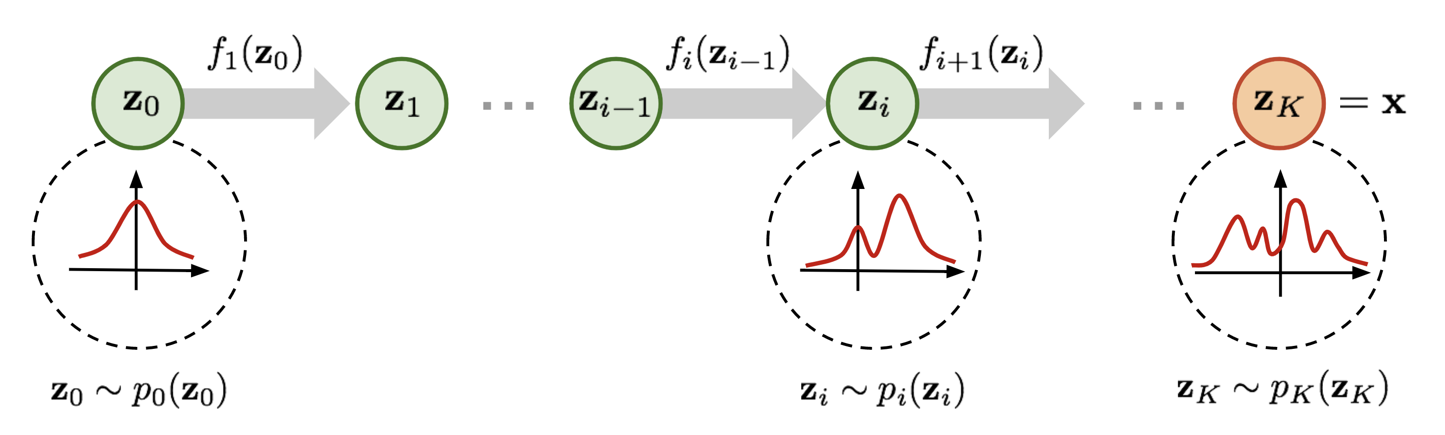
As defined in Fig. 2,
Next, let’s rewrite the equation as a function of $\mathbf{z}_i$ so that we can perform inference using the base distribution.
(*) A note on the “inverse function theorem”: If $y=f(x)$ and $x=f^{-1}(y)$, then we have:
(*) A note on “Jacobians of invertible function”: The determinant of the inverse of an invertible matrix is the inverse of the determinant: $\det(M^{-1}) = (\det(M))^{-1}$, because $\det(M)\det(M^{-1}) = \det(M \cdot M^{-1}) = \det(I) = 1$.
Given such a chain of probability density functions, we know the relationship between each pair of consecutive variables. We can expand the expression for the output $\mathbf{x}$ step by step until we trace back to the initial distribution $\mathbf{z}_0$.
The path traversed by the random variables $\mathbf{z}_i = f_i(\mathbf{z}_{i-1})$ is the flow and the full chain formed by the successive distributions $\pi_i$ is called a normalizing flow. As required by the computation in the equation, a transformation function $f_i$ should satisfy two properties:
- It is easily invertible.
- Its Jacobian determinant is easy to compute.
Models with Normalizing Flows
With normalizing flows in our toolbox, the exact log-likelihood of input data $\log p(\mathbf{x})$ becomes tractable. As a result, the training criterion for a flow-based generative model is simply the negative log-likelihood (NLL) over the training dataset $\mathcal{D}$:
RealNVP
The RealNVP (Real-valued Non-Volume Preserving; Dinh et al., 2017) model implements a normalizing flow by stacking a sequence of invertible bijective transformation functions. In each bijection $f: \mathbf{x} \mapsto \mathbf{y}$, known as an affine coupling layer, the input dimensions are split into two parts:
- The first $d$ dimensions remain the same;
- The second part, dimensions $d+1$ to $D$, undergoes an affine transformation (“scale-and-shift”), and both the scale and shift parameters are functions of the first $d$ dimensions.
where $s(.)$ and $t(.)$ are scale and translation functions, and both map $\mathbb{R}^d \mapsto \mathbb{R}^{D-d}$. The $\odot$ operation is the element-wise product.
Now let’s check whether this transformation satisfies the two basic properties required for a flow transformation.
Condition 1: “It is easily invertible.”
Yes, and it is fairly straightforward.
Condition 2: “Its Jacobian determinant is easy to compute.”
Yes. It is not hard to derive the Jacobian matrix and determinant of this transformation. The Jacobian is a lower triangular matrix.
Therefore, the determinant is simply the product of the diagonal terms.
So far, the affine coupling layer looks perfect for constructing a normalizing flow :)
Even better, because (i) computing $f^-1$ does not require computing the inverse of $s$ or $t$, and (ii) computing the Jacobian determinant does not involve computing the Jacobian of $s$ or $t$, these functions can be arbitrarily complex; that is, both $s$ and $t$ can be modeled by deep neural networks.
In one affine coupling layer, some dimensions (channels) remain unchanged. To ensure that all inputs have a chance to be altered, the model reverses the ordering in each layer so that different components are left unchanged. Following this alternating pattern, the set of units that remain identical in one transformation layer is always modified in the next. Batch normalization has been found to help train models with a very deep stack of coupling layers.
Furthermore, RealNVP can use a multi-scale architecture to build a more efficient model for large inputs. The multi-scale architecture applies several “sampling” operations to standard affine layers, including spatial checkerboard pattern masking, a squeezing operation, and channel-wise masking. Read the paper for more details on the multi-scale architecture.
NICE
The NICE (Non-linear Independent Component Estimation; Dinh, et al. 2015) model is a predecessor of RealNVP. The transformation in NICE is the affine coupling layer without the scale term, known as an additive coupling layer.
Glow
The Glow (Kingma and Dhariwal, 2018) model extends earlier reversible generative models, NICE and RealNVP, and simplifies the architecture by replacing the reverse permutation operation on channel ordering with invertible 1x1 convolutions.
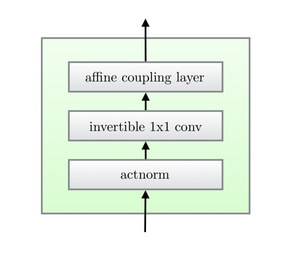
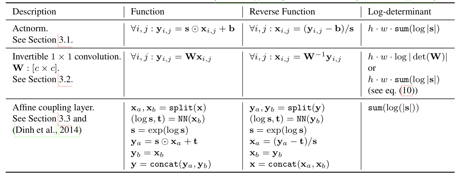
There are three substeps in one step of flow in Glow.
Substep 1: Activation normalization (short for “actnorm”)
It performs an affine transformation using a scale and bias parameter per channel, similar to batch normalization, but it works with a mini-batch size of 1. The parameters are trainable but initialized so that the first minibatch of data has mean 0 and standard deviation 1 after actnorm.
Substep 2: Invertible 1x1 conv
Between layers in the RealNVP flow, the ordering of channels is reversed so that all data dimensions have a chance to be altered. A 1×1 convolution with an equal number of input and output channels is a generalization of any permutation of the channel ordering.
Suppose we have an invertible 1x1 convolution applied to an input $h \times w \times c$ tensor $\mathbf{h}$ with a weight matrix $\mathbf{W}$ of size $c \times c$. The output is an $h \times w \times c$ tensor, denoted as $f = \texttt{conv2d}(\mathbf{h}; \mathbf{W})$. To apply the change-of-variables rule, we need to compute the Jacobian determinant $\vert \det\partial f / \partial\mathbf{h}\vert$.
Both the input and output of the 1x1 convolution here can be viewed as a matrix of size $h \times w$. Each entry $\mathbf{x}_{ij}$ ($i=1,\dots,h, j=1,\dots,w$) in $\mathbf{h}$ is a vector of $c$ channels, and each entry is multiplied by the weight matrix $\mathbf{W}$ to obtain the corresponding entry $\mathbf{y}_{ij}$ in the output matrix. The derivative of each entry is $\partial \mathbf{x}_{ij} \mathbf{W} / \partial\mathbf{x}_{ij} = \mathbf{W}$, and there are $h \times w$ such entries in total:
The inverse 1x1 convolution depends on the inverse matrix $\mathbf{W}^{-1}$. Since the weight matrix is relatively small, the computational cost of the matrix determinant (tf.linalg.det) and inversion (tf.linalg.inv) remains manageable.
Substep 3: Affine coupling layer
The design is the same as in RealNVP.
Models with Autoregressive Flows
The autoregressive constraint is a way to model sequential data, $\mathbf{x} = [x_1, \dots, x_D]$: each output depends only on data observed in the past, not on future values. In other words, the probability of observing $x_i$ is conditioned on $x_1, \dots, x_{i-1}$, and the product of these conditional probabilities gives the probability of observing the full sequence:
How you model the conditional density is up to you. It can be a univariate Gaussian with mean and standard deviation computed as functions of $x_{1:i-1}$, or a multilayer neural network with $x_{1:i-1}$ as the input.
If a flow transformation in a normalizing flow is framed as an autoregressive model, where each dimension in a vector variable is conditioned on the previous dimensions, this is an autoregressive flow.
This section starts with several classic autoregressive models (MADE, PixelRNN, WaveNet), and then we dive into autoregressive flow models (MAF and IAF).
MADE
MADE (Masked Autoencoder for Distribution Estimation; Germain et al., 2015) is a specially designed architecture that enforces the autoregressive property in an autoencoder efficiently. When using an autoencoder to predict conditional probabilities, rather than feeding the autoencoder inputs with different observation windows $D$ times, MADE removes the contribution from certain hidden units by multiplying binary mask matrices so that each input dimension is reconstructed only from previous dimensions in a given ordering in a single pass.
In a multilayer fully connected neural network, suppose we have $L$ hidden layers with weight matrices $\mathbf{W}^1, \dots, \mathbf{W}^L$ and an output layer with weight matrix $\mathbf{V}$. The output $\hat{\mathbf{x}}$ has each dimension $\hat{x}_i = p(x_i\vert x_{1:i-1})$.
Without any mask, the computation through layers looks like the following:
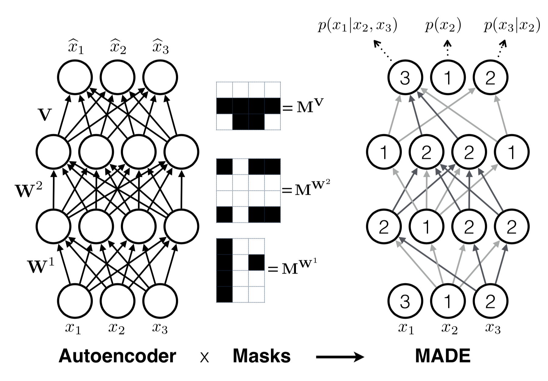
To zero out some connections between layers, we can simply multiply each weight matrix element-wise by a binary mask matrix. Each hidden node is assigned a random “connectivity integer” between $1$ and $D-1$; the assigned value for the $k$-th unit in the $l$-th layer is denoted by $m^l_k$. The binary mask matrix is determined by comparing the values of two nodes in two layers element-wise.
A unit in the current layer can only connect to units with equal or smaller numbers in the previous layer, and this type of dependency easily propagates through the network up to the output layer. Once the numbers are assigned to all units and layers, the ordering of input dimensions is fixed, and the conditional probability is produced with respect to it. See a great illustration in To ensure that all hidden units are connected to the input and output layers through some paths, $m^l_k$ is sampled to be equal to or greater than the minimal connectivity integer in the previous layer, $\min_{k’} m_{k’}^{l-1}$.
MADE training can be further facilitated by:
- Order-agnostic training: shuffle the input dimensions so that MADE can model any arbitrary ordering; this can create an ensemble of autoregressive models at runtime.
- Connectivity-agnostic training: to avoid tying a model to a specific connectivity-pattern constraint, resample $m^l_k$ for each training minibatch.
PixelRNN
PixelRNN (Oord et al, 2016) is a deep generative model for images. The image is generated one pixel at a time, and each new pixel is sampled conditional on the pixels that have already been seen.
Let’s consider an image of size $n \times n$, $\mathbf{x} = \{x_1, \dots, x_{n^2}\}$. The model starts generating pixels from the top-left corner, moving left to right and top to bottom (see Fig. 6).
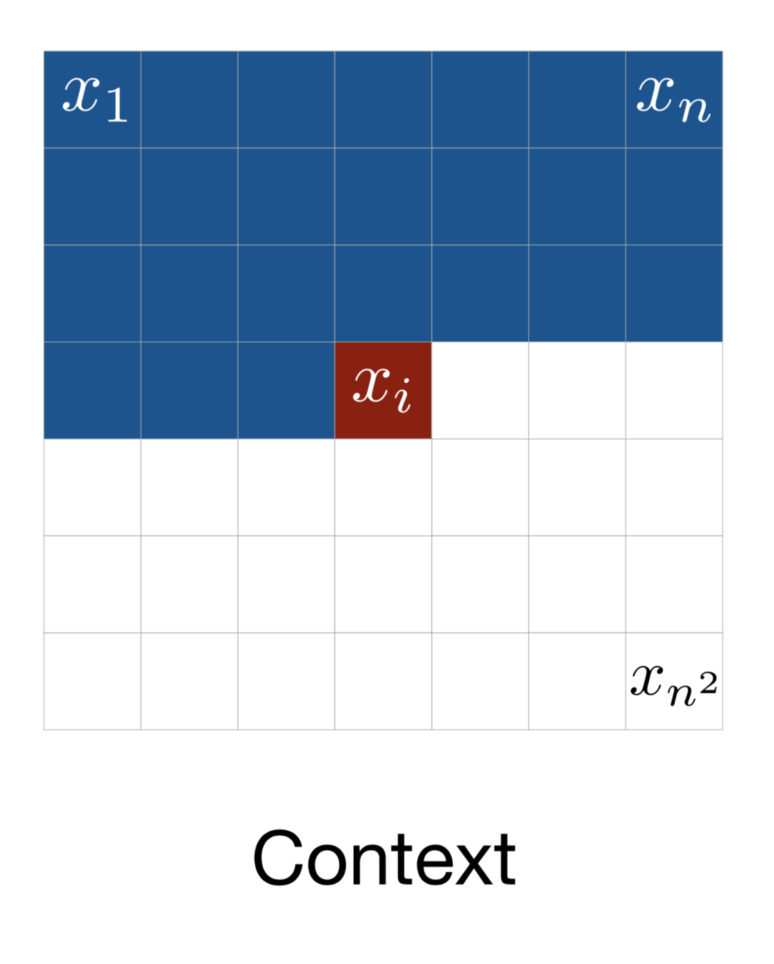
Each pixel $x_i$ is sampled from a probability distribution conditioned on the past context: pixels above it, or to its left when it is in the same row. The definition of such context looks fairly arbitrary, because how visual attention attention is applied to an image is more flexible. Somehow, a generative model with such a strong assumption works.
One implementation that can capture the entire context is the Diagonal BiLSTM. First, apply the skewing operation by offsetting each row of the input feature map by one position relative to the previous row, so that computation for each row can be parallelized. Then the LSTM states are computed with respect to the current pixel and the pixels to the left.
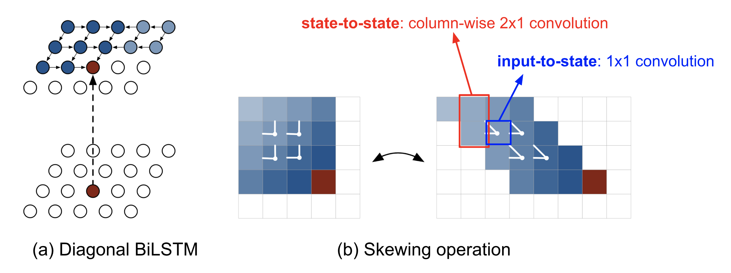
where $\circledast$ denotes the convolution operation and $\odot$ denotes element-wise multiplication. The input-to-state component $\mathbf{K}^{is}$ is a 1x1 convolution, while the state-to-state recurrent component is computed via a column-wise convolution $\mathbf{K}^{ss}$ with a 2x1 kernel.
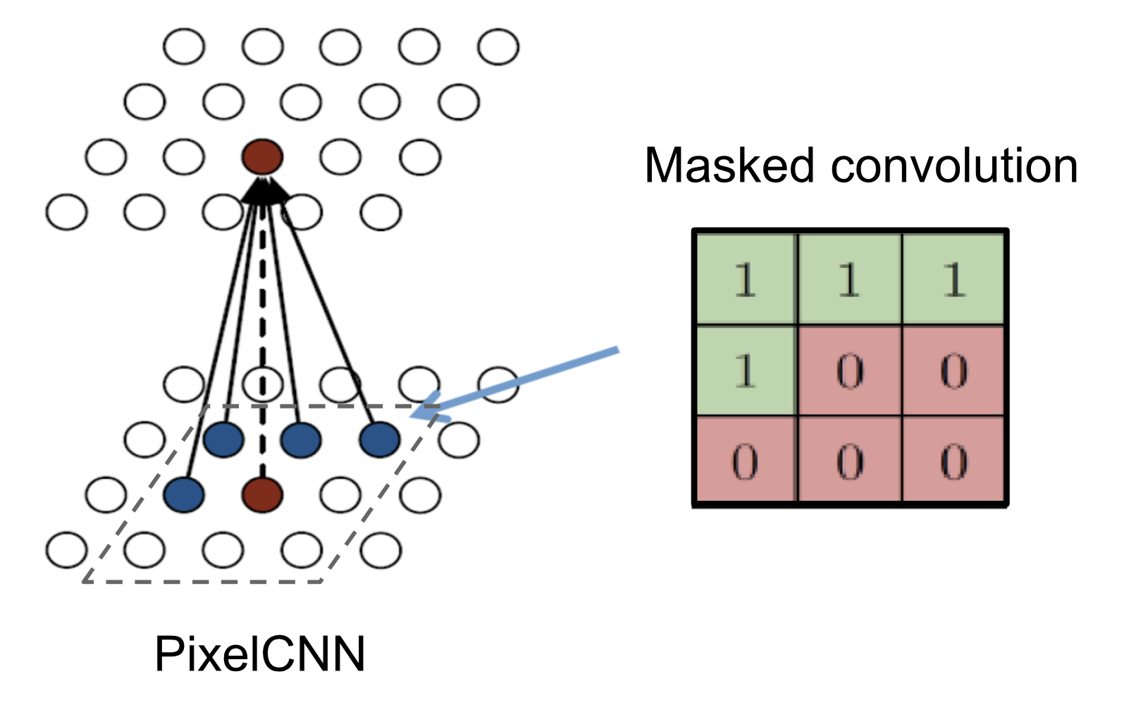
The diagonal BiLSTM layers can process an unbounded context field, but they are expensive to compute due to the sequential dependency between states. A faster implementation uses multiple convolutional layers without pooling to define a bounded context box. The convolution kernel is masked so that future context is not visible, similar to MADE. This convolutional version is called PixelCNN.
WaveNet
WaveNet (Van Den Oord, et al. 2016) is very similar to PixelCNN, but it is applied to 1-D audio signals. WaveNet consists of a stack of causal convolution, which is a convolution operation designed to respect ordering: the prediction at a given timestamp can only consume data observed in the past, with no dependence on the future. In PixelCNN, causal convolution is implemented using a masked convolution kernel. In WaveNet, causal convolution is implemented by shifting the output forward by a number of timestamps so that the output is aligned with the last input element.
One major drawback of a convolution layer is its very limited receptive field size. The output can hardly depend on inputs from hundreds or thousands of timesteps earlier, which can be a crucial requirement for modeling long sequences. WaveNet therefore adopts dilated convolution (animation), where the kernel is applied to an evenly distributed subset of samples within a much larger receptive field of the input.
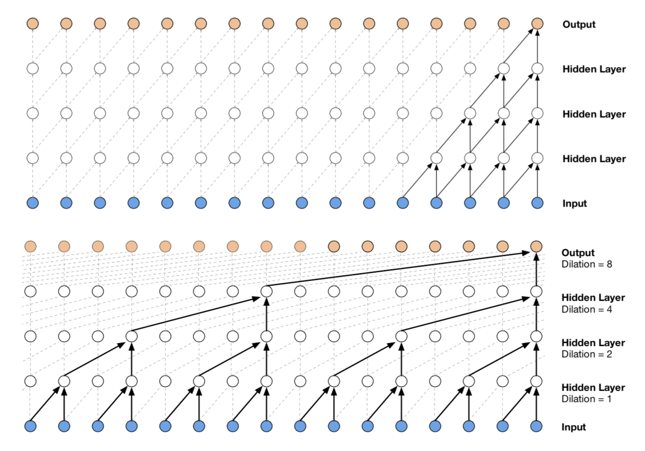
WaveNet uses the gated activation unit as the non-linear layer, as it has been found to work significantly better than ReLU for modeling 1-D audio data. The residual connection is applied after the gated activation.
where $\mathbf{W}_{f,k}$ and $\mathbf{W}_{g,k}$ are the convolution filter and gate weight matrix of the $k$-th layer, respectively; both are learnable.
Masked Autoregressive Flow
Masked Autoregressive Flow (MAF; Papamakarios et al., 2017) is a type of normalizing flow in which the transformation layer is constructed as an autoregressive neural network. MAF is very similar to Inverse Autoregressive Flow (IAF), introduced later. See further discussion of the relationship between MAF and IAF in the next section.
Given two random variables, $\mathbf{z} \sim \pi(\mathbf{z})$ and $\mathbf{x} \sim p(\mathbf{x})$, where the probability density function $\pi(\mathbf{z})$ is known, MAF aims to learn $p(\mathbf{x})$. MAF generates each $x_i$ conditioned on the preceding dimensions $\mathbf{x}_{1:i-1}$.
Specifically, the conditional probability is an affine transformation of $\mathbf{z}$, where the scale and shift terms are functions of the observed portion of $\mathbf{x}$.
- Data generation, producing a new $\mathbf{x}$:
$x_i \sim p(x_i\vert\mathbf{x}_{1:i-1}) = z_i \odot \sigma_i(\mathbf{x}_{1:i-1}) + \mu_i(\mathbf{x}_{1:i-1})\text{, where }\mathbf{z} \sim \pi(\mathbf{z})$
- Density estimation, given a known $\mathbf{x}$:
$p(\mathbf{x}) = \prod_{i=1}^D p(x_i\vert\mathbf{x}_{1:i-1})$
The generation procedure is sequential, so it is slow by design. In contrast, density estimation requires only one pass through the network using an architecture such as MADE. The transformation function is trivial to invert, and the Jacobian determinant is also easy to compute.
Inverse Autoregressive Flow
Similar to MAF, Inverse autoregressive flow (IAF; Kingma et al., 2016) also models the conditional probability of the target variable as an autoregressive model, but with a reversed flow, thereby achieving a much more efficient sampling process.
First, let’s reverse the affine transformation in MAF:
If we let:
Then we would have,
IAF aims to estimate the probability density function of $\tilde{\mathbf{x}}$, given that $\tilde{\pi}(\tilde{\mathbf{z}})$ is already known. The inverse flow is also an autoregressive affine transformation, as in MAF, but the scale and shift terms are autoregressive functions of observed variables from the known distribution $\tilde{\pi}(\tilde{\mathbf{z}})$. See the comparison between MAF and IAF in
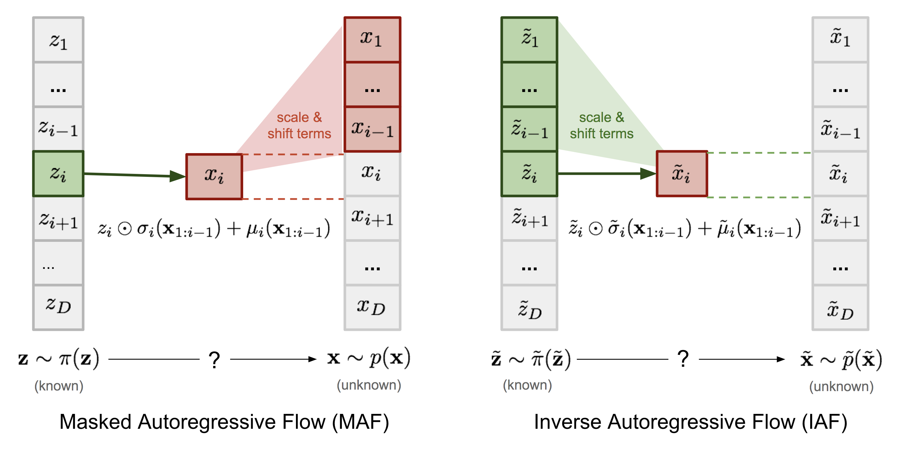
Computations of the individual elements $\tilde{x}_i$ do not depend on one another, so they are easily parallelizable (only one pass using MADE). Density estimation for a known $\tilde{\mathbf{x}}$ is not efficient, because we must recover the value of $\tilde{z}_i$ sequentially: $\tilde{z}_i = (\tilde{x}_i - \tilde{\mu}_i(\tilde{\mathbf{z}}_{1:i-1})) / \tilde{\sigma}_i(\tilde{\mathbf{z}}_{1:i-1})$, for a total of D times.
| Base distribution | Target distribution | Model | Data generation | Density estimation | |
|---|---|---|---|---|---|
| MAF | $\mathbf{z}\sim\pi(\mathbf{z})$ | $\mathbf{x}\sim p(\mathbf{x})$ | $x_i = z_i \odot \sigma_i(\mathbf{x}_{1:i-1}) + \mu_i(\mathbf{x}_{1:i-1})$ | Sequential; slow | One pass; fast |
| IAF | $\tilde{\mathbf{z}}\sim\tilde{\pi}(\tilde{\mathbf{z}})$ | $\tilde{\mathbf{x}}\sim\tilde{p}(\tilde{\mathbf{x}})$ | $\tilde{x}_i = \tilde{z}_i \odot \tilde{\sigma}_i(\tilde{\mathbf{z}}_{1:i-1}) + \tilde{\mu}_i(\tilde{\mathbf{z}}_{1:i-1})$ | One pass; fast | Sequential; slow |
| ----- | ----- | ----- | ----- | ----- | ----- |
VAE + Flows
In Variational Autoencoder, if we want to model the posterior $p(\mathbf{z}\vert\mathbf{x})$ as a more complex distribution rather than a simple Gaussian, we can intuitively use a normalizing flow to transform the base Gaussian for better density approximation. The encoder would then predict a set of scale and shift terms $(\mu_i, \sigma_i)$, all of which are functions of the input $\mathbf{x}$. Read the paper for more details if you are interested.
If you notice mistakes or errors in this post, please do not hesitate to contact me at [lilian dot wengweng at gmail dot com], and I will be very happy to correct them right away!
See you in the next post :D
Cited as:
@article{weng2018flow,
  title   = "Flow-based Deep Generative Models",
  author  = "Weng, Lilian",
  journal = "lilianweng.github.io",
  year    = "2018",
  url     = "https://lilianweng.github.io/posts/2018-10-13-flow-models/"
}
Reference
[1] Danilo Jimenez Rezende, and Shakir Mohamed. “Variational inference with normalizing flows.” ICML 2015.
[2] Normalizing Flows Tutorial, Part 1: Distributions and Determinants by Eric Jang.
[3] Normalizing Flows Tutorial, Part 2: Modern Normalizing Flows by Eric Jang.
[4] Normalizing Flows by Adam Kosiorek.
[5] Laurent Dinh, Jascha Sohl-Dickstein, and Samy Bengio. “Density estimation using Real NVP.” ICLR 2017.
[6] Laurent Dinh, David Krueger, and Yoshua Bengio. “NICE: Non-linear independent components estimation.” ICLR 2015 Workshop track.
[7] Diederik P. Kingma, and Prafulla Dhariwal. “Glow: Generative flow with invertible 1x1 convolutions.” arXiv:1807.03039 (2018).
[8] Germain, Mathieu, Karol Gregor, Iain Murray, and Hugo Larochelle. “Made: Masked autoencoder for distribution estimation.” ICML 2015.
[9] Aaron van den Oord, Nal Kalchbrenner, and Koray Kavukcuoglu. “Pixel recurrent neural networks.” ICML 2016.
[10] Diederik P. Kingma, et al. “Improved variational inference with inverse autoregressive flow.” NIPS. 2016.
[11] George Papamakarios, Iain Murray, and Theo Pavlakou. “Masked autoregressive flow for density estimation.” NIPS 2017.
[12] Jianlin Su, and Guang Wu. “f-VAEs: Improve VAEs with Conditional Flows.” arXiv:1809.05861 (2018).
[13] Van Den Oord, Aaron, et al. “WaveNet: A generative model for raw audio.” SSW. 2016.