Generalized Language Models
[Updated on 2019-02-14: add ULMFiT and GPT-2.] [Updated on 2020-02-29: add ALBERT.] [Updated on 2020-10-25: add RoBERTa.] [Updated on 2020-12-13: add T5.] [Updated on 2020-12-30: add GPT-3.] [Updated on 2021-11-13: add XLNet, BART and ELECTRA; Also updated the Summary section.] Are they ELMo and BERT, (Image source: here) We saw remarkable progress in NLP in 2018. Large-scale, pre-trained language models such as OpenAI GPT and BERT delivered strong results across a broad range of language tasks while relying on generic model architectures. This concept parallels how ImageNet classification pre-training benefits many vision tasks (*). However, unlike vision classification pre-training, this straightforward and effective NLP approach does not require labeled data during pre-training, which lets us push training scale and explore larger experiments, up to our practical limits.
· 36 min read · Curated and presented by Arthur Sedek
As a follow-up to the post on word embeddings, this article discusses models for learning contextualized word vectors, along with the emerging trend of large, unsupervised, pre-trained language models. These approaches have delivered remarkable state-of-the-art results across a wide range of language tasks.
[Updated on 2019-02-14: add ULMFiT and GPT-2.]
[Updated on 2020-02-29: add ALBERT.]
[Updated on 2020-10-25: add RoBERTa.]
[Updated on 2020-12-13: add T5.]
[Updated on 2020-12-30: add GPT-3.]
[Updated on 2021-11-13: add XLNet, BART and ELECTRA; Also updated the Summary section.]

NLP saw striking progress in 2018. Large-scale pre-trained language models such as OpenAI GPT and BERT achieved strong performance across many language tasks using broadly applicable model architectures. The underlying intuition mirrors the way ImageNet classification pre-training benefits many vision tasks (*). In NLP, this approach can be even more advantageous than vision classification pre-training because it does not require labeled data for pre-training. As a result, we can push training scale as far as resources allow.
(*) He et al. (2018) found that pre-training might not be necessary for image segmentation task.
In my earlier NLP post on word embedding, the embeddings described are not context-specific. They are learned from word concurrency rather than sequential context. Consequently, in the sentences “I am eating an apple” and “I have an Apple phone”, the two occurrences of “apple” refer to very different concepts, yet they would still share the same embedding vector.
Even so, early practical uses of word embeddings often treated them as extra features for an existing task-specific model, and in that setup the potential gains are inherently limited.
In this post, we examine multiple approaches designed to make embeddings context-dependent and to reduce the cost and complexity of applying them to downstream tasks in a more general form.
CoVe
CoVe (McCann et al. 2017), short for Contextual Word Vectors, is a type of word embedding learned by the encoder of an attentional seq-to-seq machine translation model. Unlike the traditional word embeddings introduced here, CoVe representations are functions of the full input sentence.
NMT Recap
The Neural Machine Translation (NMT) system here consists of a standard two-layer bidirectional LSTM encoder and an attentional two-layer unidirectional LSTM decoder. It is pre-trained on the English-German translation task. The encoder learns and optimizes embedding vectors for English words so that they can be translated into German. The motivating intuition is that, before transforming words into another language, the encoder must capture high-level semantic and syntactic information. Therefore, the encoder outputs can be repurposed as contextualized word embeddings for a variety of downstream language tasks.
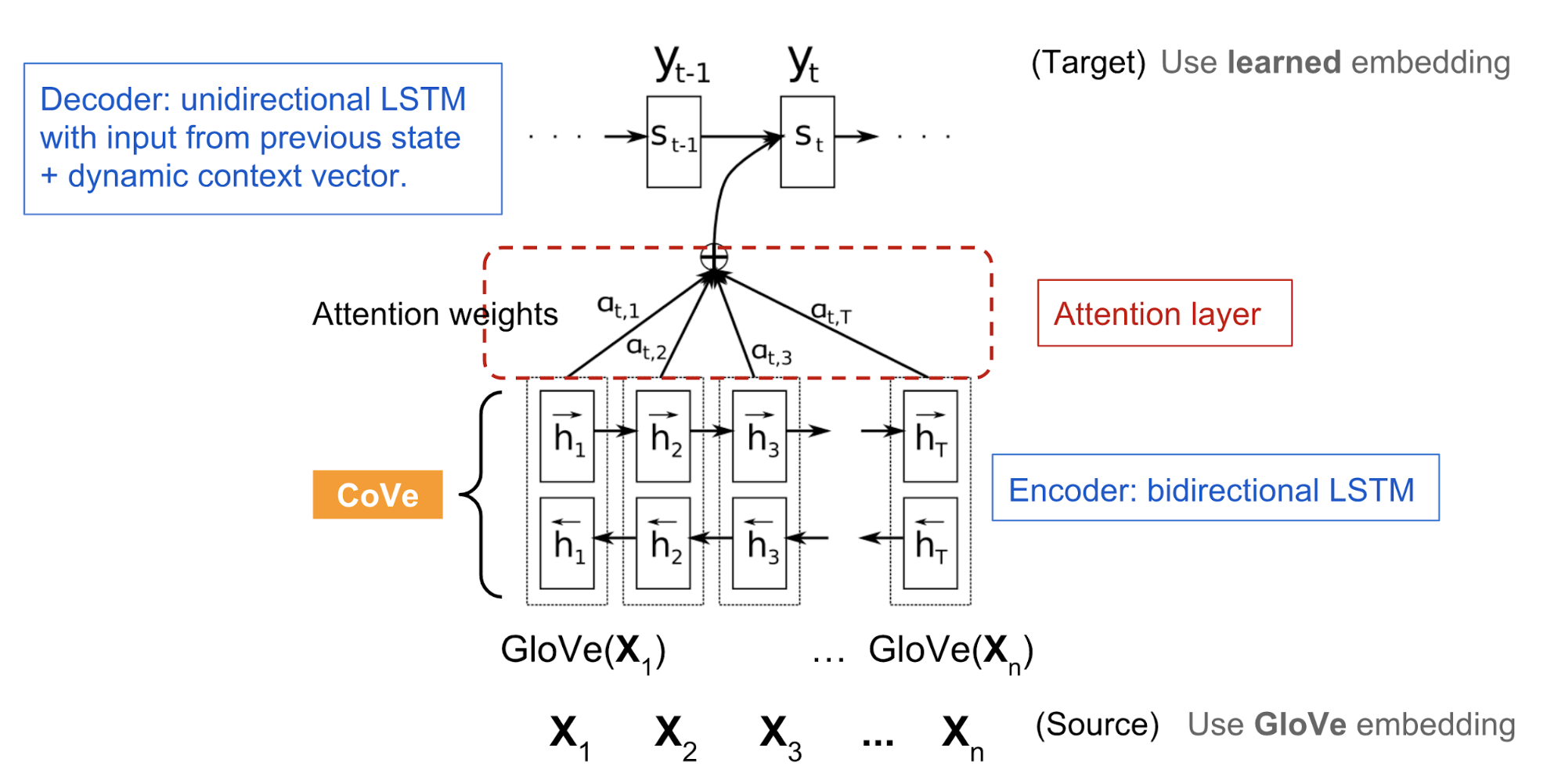
- A sequence of $n$ words in source language (English): $x = [x_1, \dots, x_n]$.
- A sequence of $m$ words in target language (German): $y = [y_1, \dots, y_m]$.
- The GloVe vectors of source words: $\text{GloVe}(x)$.
- Randomly initialized embedding vectors of target words: $z = [z_1, \dots, z_m]$.
- The biLSTM encoder outputs a sequence of hidden states: $h = [h_1, \dots, h_n] = \text{biLSTM}(\text{GloVe}(x))$ and $h_t = [\overrightarrow{h}_t; \overleftarrow{h}_t]$ where the forward LSTM computes $\overrightarrow{h}_t = \text{LSTM}(x_t, \overrightarrow{h}_{t-1})$ and the backward computation gives us $\overleftarrow{h}_t = \text{LSTM}(x_t, \overleftarrow{h}_{t-1})$.
- The attentional decoder outputs a distribution over words: $p(y_t \mid H, y_1, \dots, y_{t-1})$ where $H$ is a stack of hidden states $\{h\}$ along the time dimension:
Use CoVe in Downstream Tasks
The hidden states produced by the NMT encoder are treated as context vectors for other language tasks:
The paper proposes using the concatenation of GloVe and CoVe for question-answering and classification tasks. GloVe is learned from ratios of global word co-occurrences and therefore does not incorporate sentence context. CoVe, in contrast, is generated by processing text sequences and can capture contextual information.
For a downstream task, we first build the concatenated GloVe + CoVe vectors for the input tokens, and then provide them to task-specific models as additional features.
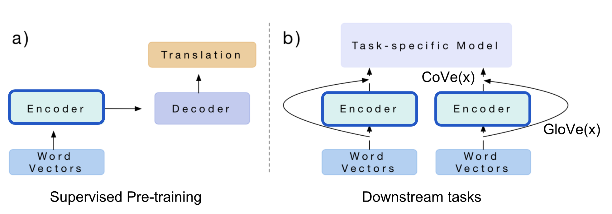
Summary: CoVe has two clear limitations: (1) pre-training is limited by the availability of supervised translation datasets; (2) CoVe’s contribution to final performance is constrained by the architecture of the task-specific model.
In the sections that follow, we will see that ELMo addresses issue (1) via unsupervised pre-training. OpenAI GPT and BERT go further by combining unsupervised pre-training with a generative model architecture that can be adapted to many downstream tasks, thereby addressing both limitations.
ELMo
ELMo, short for Embeddings from Language Model (Peters, et al, 2018), learns contextualized word representations by pre-training a language model in an unsupervised manner.
Bidirectional Language Model
The bidirectional Language Model (biLM) is the core component of ELMo. Given an input sequence of $n$ tokens, $(x_1, \dots, x_n)$, the language model is trained to predict the probability of the next token conditioned on the history.
In the forward direction, the history consists of tokens that precede the target token:
In the backward direction, the history consists of tokens that follow the target token:
Predictions in both directions are modeled using multi-layer LSTMs, with hidden states $\overrightarrow{\mathbf{h}}_{i,\ell}$ and $\overleftarrow{\mathbf{h}}_{i,\ell}$ for input token $x_i$ at the layer level $\ell=1,\dots,L$. The final layer hidden state $\mathbf{h}_{i,L} = [\overrightarrow{\mathbf{h}}_{i,L}; \overleftarrow{\mathbf{h}}_{i,L}]$ is used to produce token probabilities after softmax normalization. The two directions share the embedding layer and the softmax layer, parameterized by $\Theta_e$ and $\Theta_s$ respectively.
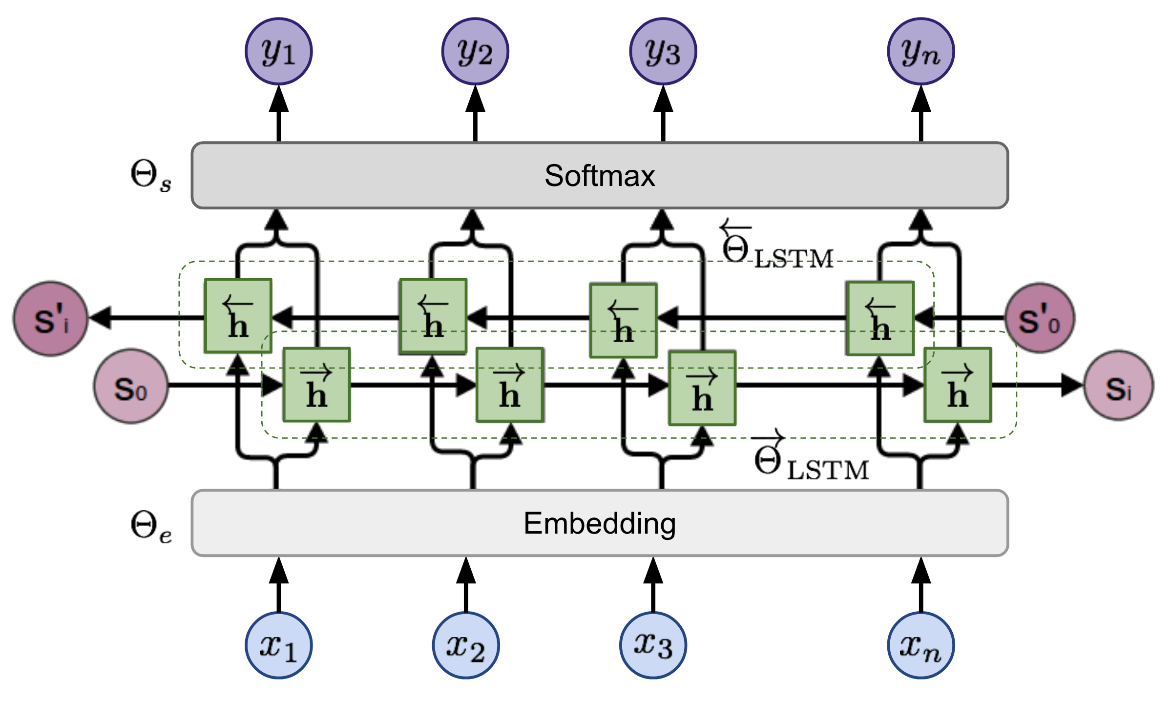
The training objective minimizes the negative log likelihood (equivalently, maximizes the log likelihood of the true words) in both directions:
ELMo Representations
Given a $L$-layer biLM, ELMo forms token representations by stacking all hidden states across layers and learning a task-specific linear combination. For token $x_i$, the representation includes $2L+1$ vectors:
where $\mathbf{h}_{0, \ell}$ is the embedding layer output and $\mathbf{h}_{i, \ell} = [\overrightarrow{\mathbf{h}}_{i,\ell}; \overleftarrow{\mathbf{h}}_{i,\ell}]$.
The linear combination weights, $\mathbf{s}^\text{task}$, are learned separately for each downstream task and normalized with softmax. The scaling factor $\gamma^\text{task}$ is introduced to correct misalignment between the distribution of biLM hidden states and the distribution of task-specific representations.
To analyze what information is captured by hidden states at different layers, ELMo evaluates representations from different biLM layers on tasks emphasizing either semantics or syntax:
- Semantic task: The word sense disambiguation (WSD) task focuses on determining a word’s meaning given context. The biLM top layer performs better on this task than the first layer.
- Syntax task: The part-of-speech (POS) tagging task aims to infer the grammatical role of a word in a sentence. Higher accuracy is achieved using the biLM first layer rather than the top layer.
This comparison suggests that lower layers tend to represent syntactic information more strongly, while higher layers capture more semantic information. Because different layers encode different types of information, stacking them together helps.
Use ELMo in Downstream Tasks
As with CoVe, ELMo embeddings can be injected into the input or lower levels of task-specific models. In addition, for some tasks (that is, SNLI and SQuAD, but not SRL), incorporating ELMo at the output level also improves results.
ELMo yields the largest gains on tasks with limited labeled data. With ELMo, comparable performance can often be achieved using substantially fewer labeled examples.
Summary: Because language model pre-training is unsupervised, it can in principle be scaled aggressively given the abundance of unlabeled text corpora. However, ELMo still depends on task-customized models, so improvements are typically incremental, and finding an effective architecture for each task remains non-trivial.
Cross-View Training
In ELMo, unsupervised pre-training and task-specific learning are performed by two independent models in two separate stages. Cross-View Training (abbr. CVT; Clark et al., 2018) merges these ideas into a unified semi-supervised procedure. In CVT, a biLSTM encoder’s representations are improved through both supervised learning on labeled data and unsupervised learning on auxiliary tasks using unlabeled data.
Model Architecture
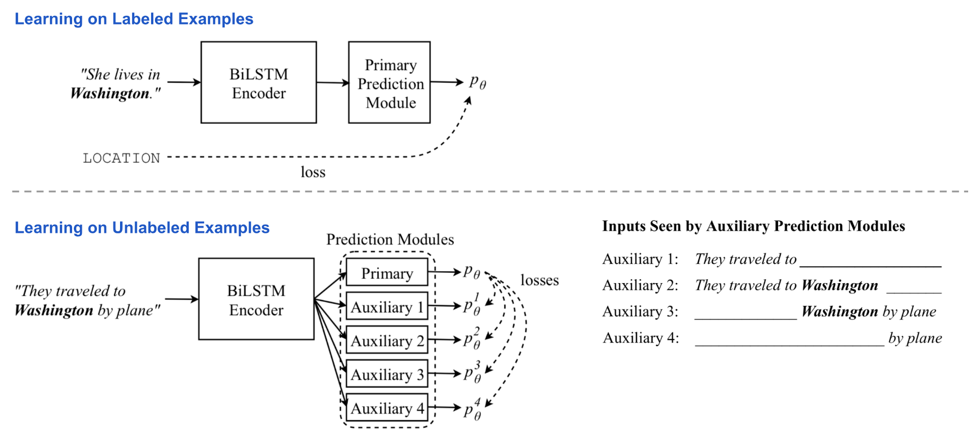
The model contains a two-layer bidirectional LSTM encoder and a primary prediction module. During training, the model alternates between batches of labeled and unlabeled examples.
- For labeled examples, all parameters are updated via standard supervised learning, using the usual cross-entropy loss.
- For unlabeled examples, the primary prediction module can still produce a “soft” target, even though its correctness is not directly observable. CVT defines auxiliary tasks in which the predictor is restricted to a limited view of the input, for example, using only encoder hidden states from a single direction. The auxiliary predictions are trained to match the primary prediction generated from the full view.
This forces the encoder to distill information from the full context into a partial representation. During this stage, gradients are backpropagated through the biLSTM encoder while the primary prediction module remains fixed. The loss minimizes the distance between auxiliary predictions and the primary “soft” target.
Multi-Task Learning
For simultaneous training on multiple tasks, CVT introduces additional primary prediction modules (one per task) while sharing a single sentence-representation encoder across all tasks. During supervised training, one task is randomly selected, and the model updates the parameters of that task’s predictor together with the shared encoder. With unlabeled examples, the encoder is optimized jointly across all tasks by minimizing, for each task, the discrepancy between auxiliary outputs and the corresponding primary prediction.
This multi-task setup encourages more general representations and also yields a useful by-product: all-tasks-labeled examples derived from unlabeled data. These labels are valuable because cross-task labels are helpful yet uncommon.
Use CVT in Downstream Tasks
In principle, the primary prediction module can take many forms, including generic designs and task-specific architectures. The CVT paper provides examples of both.
For sequential tagging tasks (token-level classification) such as NER or POS tagging, the predictor consists of two fully connected layers followed by a softmax that produces a probability distribution over class labels. For each token $\mathbf{x}_i$, we use the corresponding hidden states from the two encoder layers, $\mathbf{h}_1^{(i)}$ and $\mathbf{h}_2^{(i)}$:
The auxiliary tasks receive only the forward or backward LSTM state from the first layer. Because these tasks observe only partial context (either left or right), they must behave similarly to a language model, attempting to predict the next token given the available context. The fwd and bwd auxiliary tasks use a single direction. The future and past tasks go one step further in the forward and backward directions, respectively.
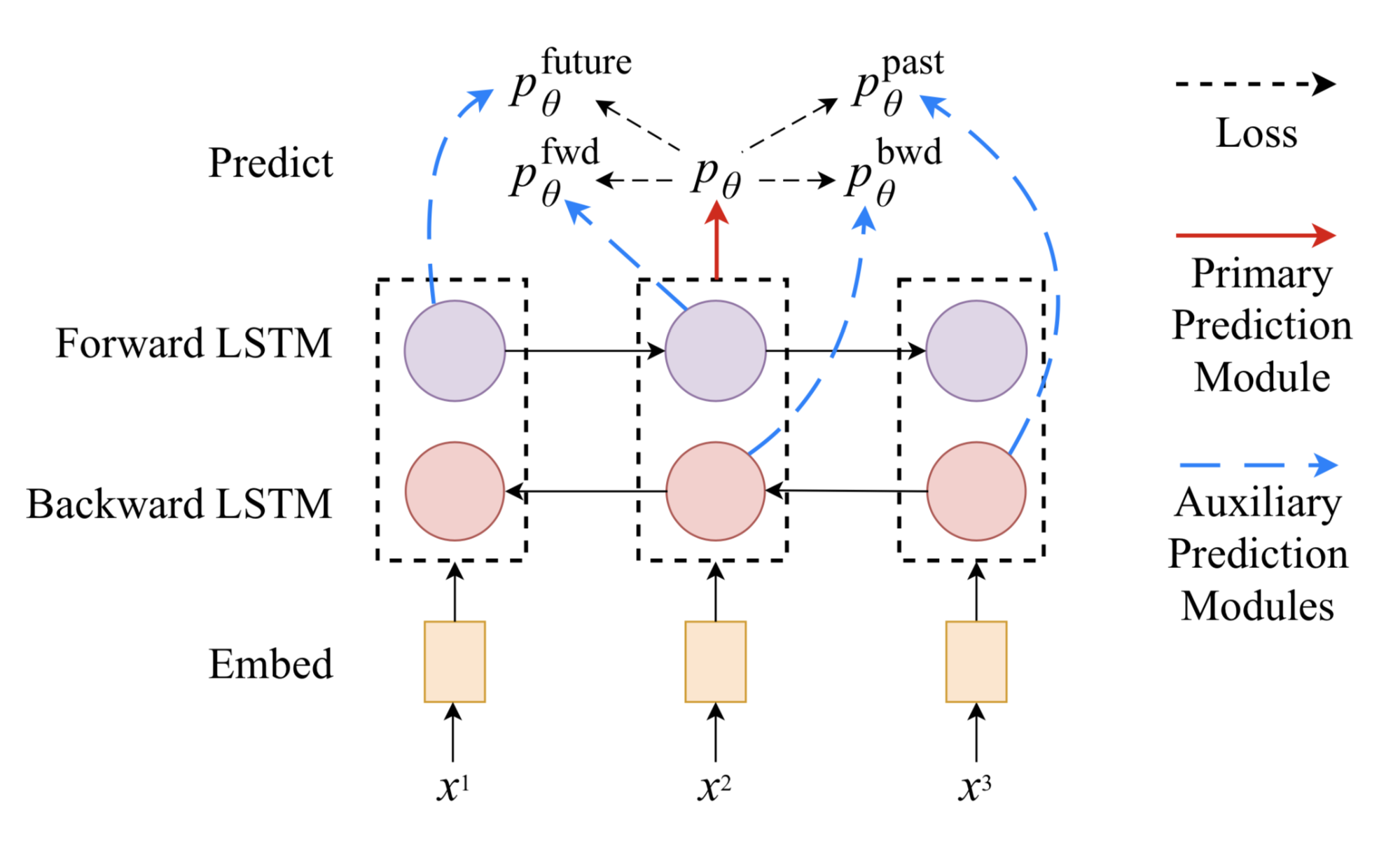
Note that when the primary prediction module includes dropout, dropout is applied normally during labeled training. However, dropout is not applied when generating the “soft” targets for auxiliary tasks during training on unlabeled examples.
For machine translation, the primary prediction module is replaced by a standard unidirectional LSTM decoder with attention. Two auxiliary tasks are used: (1) apply dropout to the attention weight vector by randomly zeroing some values; (2) predict a future word in the target sequence. The primary prediction that auxiliary tasks must match is the best predicted target sequence obtained by running the fixed primary decoder on the input sequence with beam search.
ULMFiT
The strategy of combining a generative pre-trained language model with task-specific fine-tuning was first explored in ULMFiT (Howard & Ruder, 2018), directly inspired by the success of ImageNet pre-training in computer vision. The underlying model is AWD-LSTM.
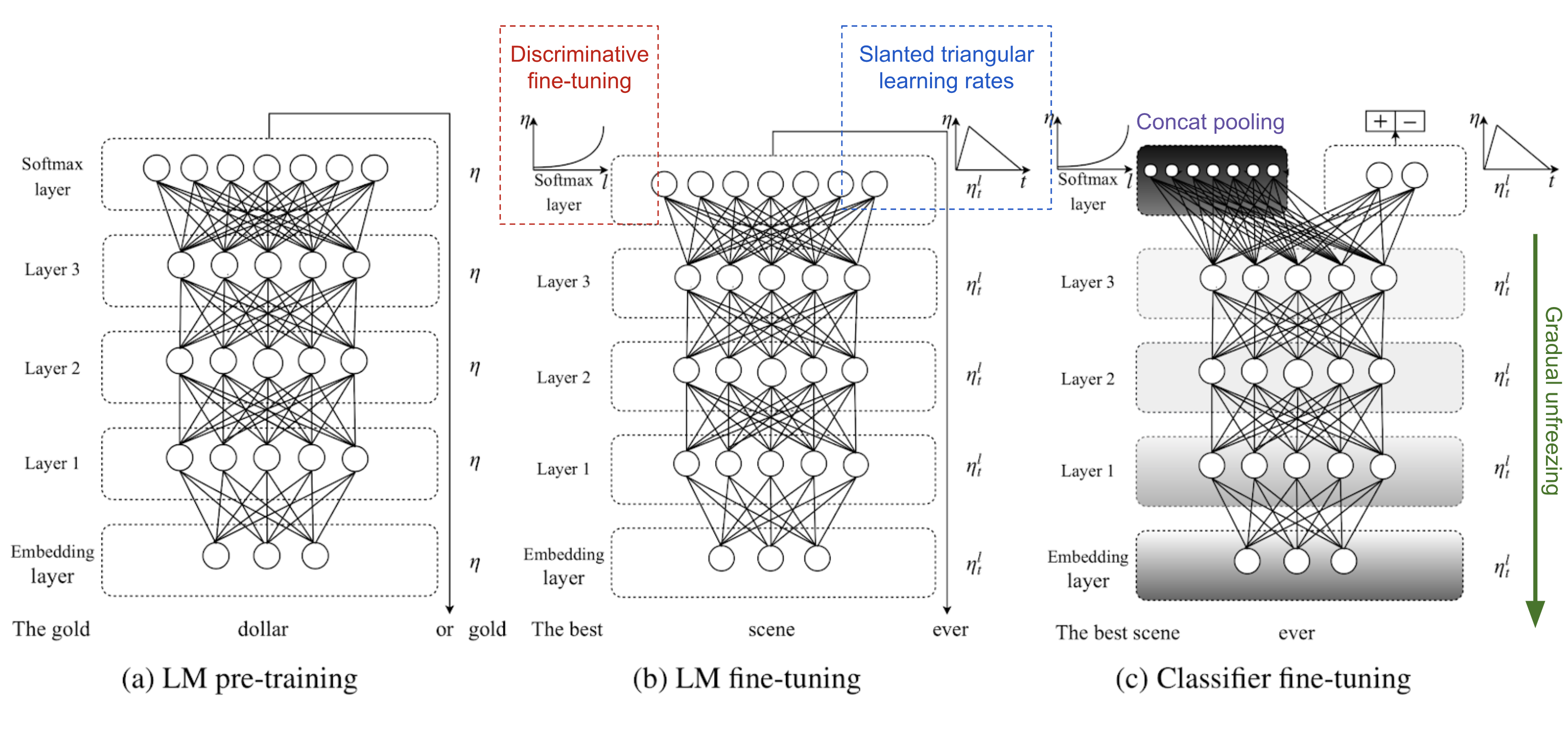
ULMFiT uses three steps to obtain strong transfer learning performance on downstream language classification tasks:
-
General LM pre-training: performed on Wikipedia text.
-
Target task LM fine-tuning: ULMFiT proposes two techniques to stabilize the fine-tuning process (described below).
-
Discriminative fine-tuning is motivated by the observation that different LM layers capture different kinds of information (see the discussion above). ULMFiT proposes tuning each layer using a different learning rate, $\{\eta^1, \dots, \eta^\ell, \dots, \eta^L\}$, where $\eta$ is the base learning rate for the first layer, $\eta^\ell$ is for the $\ell$-th layer, and there are $L$ layers in total.
-
Slanted triangular learning rates (STLR) define a learning-rate schedule that increases linearly at first and then decreases linearly. The warm-up increase is brief so the model can quickly reach a parameter region suitable for the task, while the longer decay phase supports more effective fine-tuning.
- Target task classifier fine-tuning: the pre-trained LM is extended with two standard feed-forward layers and a final softmax to predict the target label distribution.
-
Concat pooling computes max-pooling and mean-pooling over the sequence of hidden states, then concatenates these pooled vectors with the final hidden state.
-
Gradual unfreezing mitigates catastrophic forgetting by progressively unfreezing layers starting from the last layer. First, the last layer is unfrozen and fine-tuned for one epoch. Next, the layer below it is unfrozen, and the process continues until all layers have been tuned.
GPT
Building on an idea similar to ELMo, OpenAI GPT, short for Generative Pre-training Transformer (Radford et al., 2018), scales unsupervised language model training substantially by using a very large collection of freely available text corpora. Despite this shared motivation, GPT differs from ELMo in two important ways.
- The architectures differ: ELMo uses a shallow concatenation of independently trained left-to-right and right-to-left multi-layer LSTMs, whereas GPT uses a multi-layer transformer decoder.
- The downstream usage differs: ELMo injects contextualized embeddings into task-specific models as additional features, whereas GPT fine-tunes the same base model for all end tasks.
Transformer Decoder as Language Model
Relative to the original transformer architecture, the transformer decoder removes the encoder portion. As a result, there is only a single input sentence rather than separate source and target sequences.
The model applies multiple transformer blocks to the embeddings of the input sequence. Each block includes a masked multi-headed self-attention layer and a pointwise feed-forward layer. After the final block, a softmax produces a distribution over target tokens.
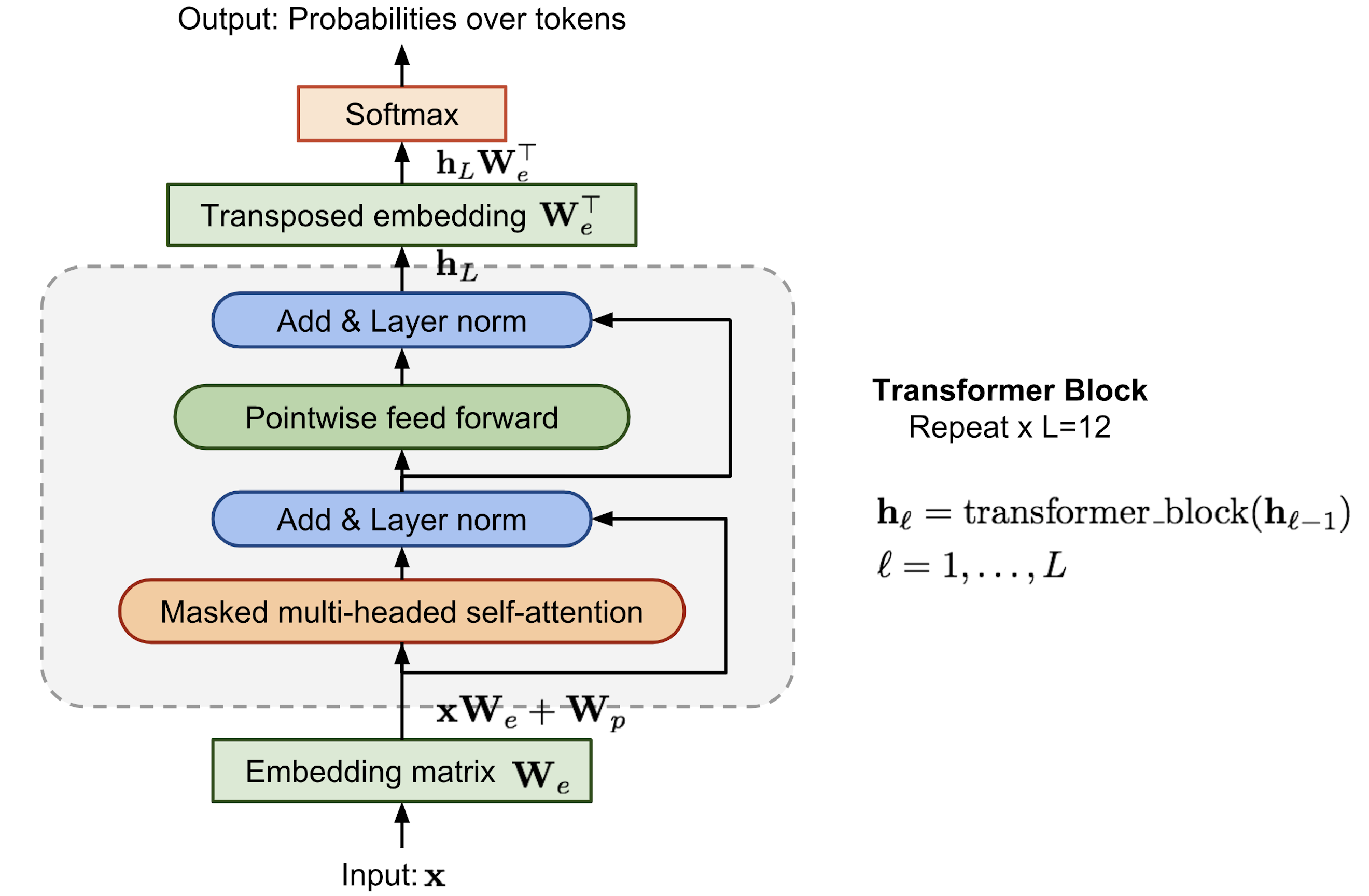
The training objective is the negative log-likelihood, as in ELMo, but it excludes the backward direction. If a context window of size $k$ appears before the target word, the loss takes the form:
Byte Pair Encoding
Byte Pair Encoding (BPE) is used to encode input sequences. BPE was originally introduced in the 1990s as a data compression method and later adopted to address the open-vocabulary problem in machine translation, where rare or unknown words are common when translating into new languages. Based on the intuition that rare and unknown words can often be decomposed into subwords, BPE searches for an effective segmentation by iteratively and greedily merging frequent pairs of characters.
Supervised Fine-Tuning
The most significant change introduced by OpenAI GPT is eliminating the task-specific model and using the pre-trained language model directly.
Consider a classification task. Suppose each labeled example contains $n$ tokens, $\mathbf{x} = (x_1, \dots, x_n)$, and one label $y$. GPT processes the input sequence $\mathbf{x}$ with the pre-trained transformer decoder. The final-layer output for the last token $x_n$ is $\mathbf{h}_L^{(n)}$. With only one additional trainable weight matrix, $\mathbf{W}_y$, GPT can then predict a distribution over class labels.

The objective is to minimize the negative log-likelihood of the true labels. In addition, it has been found beneficial to include the language model (LM) loss as an auxiliary term, because:
- (1) it can speed up convergence during training; and
- (2) it is expected to improve the supervised model’s generalization.
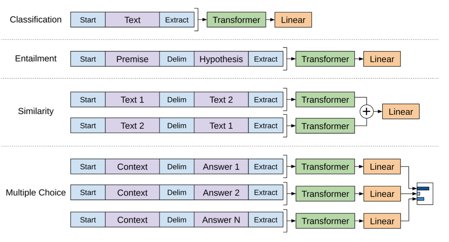
With a similar setup, other downstream tasks do not require a customized model architecture (see Fig. 7). When the task input includes multiple sentences, a special delimiter token ($) is inserted between each sentence pair. The embedding for this delimiter is an additional parameter to learn, but the overhead should be minimal.
For the sentence similarity task, because sentence order is irrelevant, both orderings are used. For the multiple-choice task, the context is paired with each answer candidate.
Summary: It is both striking and encouraging that such a general framework was able to surpass state of the art on most language tasks at the time (June 2018). In the first stage, generative pre-training of a language model can absorb as much free text as possible. In the second stage, the model is fine-tuned for specific tasks using a small labeled dataset and only a minimal number of new parameters.
One limitation of GPT is its unidirectional nature: the model is trained only to predict future context from left to right.
BERT
BERT, short for Bidirectional Encoder Representations from Transformers (Devlin, et al., 2019), is a direct descendant of GPT: it trains a large language model on free text and then fine-tunes it on specific tasks without requiring task-specific network architectures.
Relative to GPT, BERT’s key change and primary improvement is bidirectional training. The model is trained to predict context on both the left and the right. According to the ablation study, the paper claimed that:
“bidirectional nature of our model is the single most important new contribution”
Pre-training Tasks
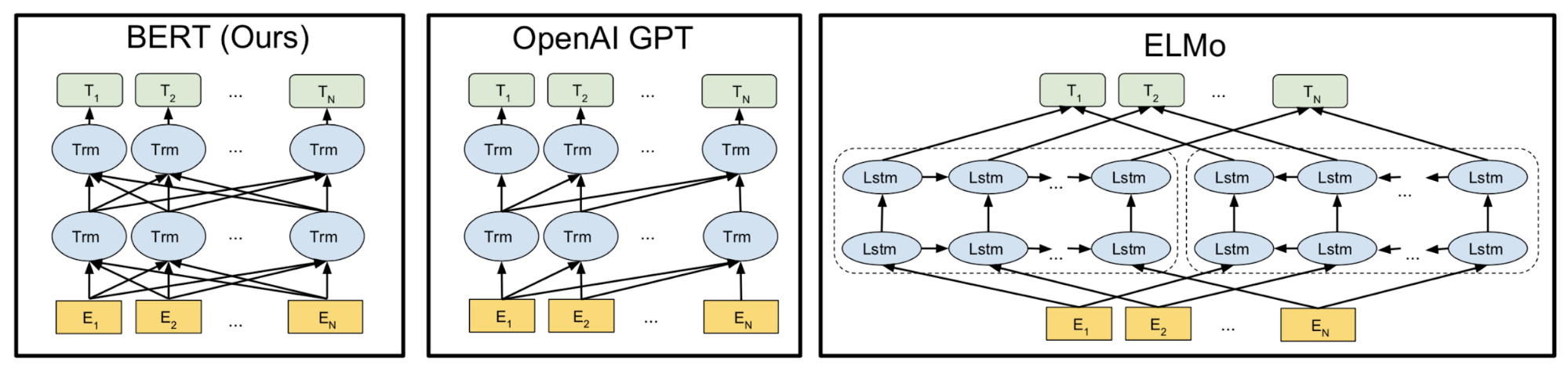
BERT uses a multi-layer bidirectional Transformer encoder as its architecture.
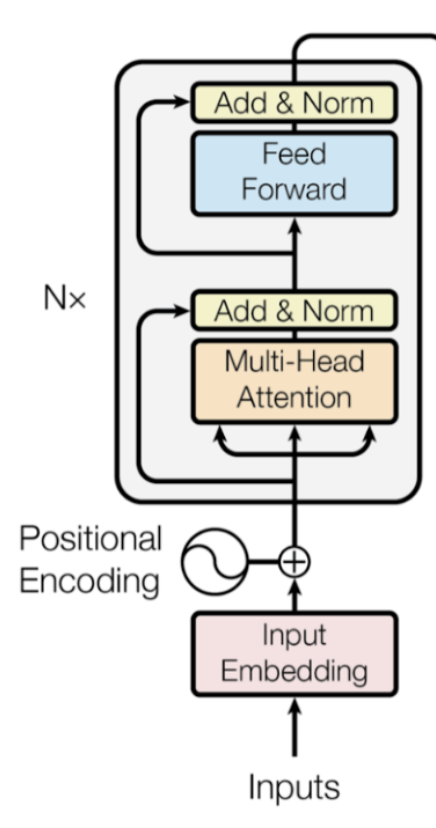
To promote bidirectional prediction and sentence-level understanding, BERT is trained with two tasks rather than the standard language modeling objective (predicting the next token given context).
*Task 1: Mask language model (MLM)
From Wikipedia: “A cloze test (also cloze deletion test) is an exercise, test, or assessment consisting of a portion of language with certain items, words, or signs removed (cloze text), where the participant is asked to replace the missing language item. … The exercise was first described by W.L. Taylor in 1953.”
It is reasonable to expect that a representation trained to model the context around a word (rather than only what follows it) can better capture the word’s meaning, both syntactically and semantically. BERT encourages this behavior by training on the mask language model task:
- Randomly mask 15% of tokens in each sequence. If masked tokens were always replaced by a special placeholder
[MASK], that token would never appear during fine-tuning. To address this, BERT uses several heuristic strategies:- (a) with 80% probability, replace the selected tokens with
[MASK]; - (b) with 10% probability, replace them with a random token;
- (c) with 10% probability, keep them unchanged.
- (a) with 80% probability, replace the selected tokens with
- The model predicts only the missing words, but it is not told which tokens have been replaced or which positions are targets. As a result, the output size is only 15% of the input size.
Task 2: Next sentence prediction
Because many downstream tasks require understanding relationships between sentences (for example, QA and NLI), BERT introduces an auxiliary objective that trains a binary classifier to determine whether one sentence follows another:
- Sample sentence pairs (A, B) such that:
- (a) 50% of the time, B follows A;
- (b) 50% of the time, B does not follow A.
- The model encodes both sentences and outputs a binary label indicating whether B is the next sentence after A.
The training data for both auxiliary tasks can be generated straightforwardly from any monolingual corpus, so the possible training scale is unbounded. The total training loss is the sum of the mean masked LM likelihood and the mean next sentence prediction likelihood.
Input Embedding
The input embedding is computed as the sum of three components:
- WordPiece tokenization embeddings: The WordPiece model was originally proposed for Japanese and Korean segmentation. Rather than relying on naturally separated English words, words can be further split into subword units, which can be more effective for handling rare or unknown terms. If you are interested in optimal splitting procedures, see the linked papers.
- Segment embeddings: When the input includes two sentences, sentence A and sentence B use different segment embeddings, and the sentences are separated by the special token
[SEP]. If the input contains only one sentence, only sentence A embeddings are used. - Position embeddings: Positional embeddings are learned instead of being hard-coded.
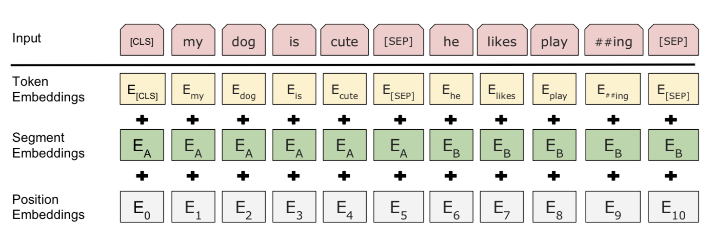
Note that the first token is always forced to be [CLS], a placeholder that is later used for prediction in downstream tasks.
Use BERT in Downstream Tasks
As with OpenAI GPT, fine-tuning BERT requires adding only a small number of new parameters.
For classification tasks, the prediction is computed by taking the final hidden state of the special first token [CLS], $\mathbf{h}^\text{[CLS]}_L$, and multiplying it by a small weight matrix, $\text{softmax}(\mathbf{h}^\text{[CLS]}_L \mathbf{W}_\text{cls})$.
For QA tasks such as SQuAD, the goal is to predict a text span in a paragraph that answers a given question. BERT predicts two token-level probability distributions that correspond to the span start and span end. Only two small matrices, $\mathbf{W}_\text{s}$ and $\mathbf{W}_\text{e}$, are newly learned during fine-tuning, and $\text{softmax}(\mathbf{h}^\text{(i)}_L \mathbf{W}_\text{s})$ and $\text{softmax}(\mathbf{h}^\text{(i)}_L \mathbf{W}_\text{e})$ define the two probability distributions.
Overall, the task-specific additions for fine-tuning are minimal: typically one or two weight matrices that map Transformer hidden states into an interpretable output. For other cases, see the paper for implementation details.
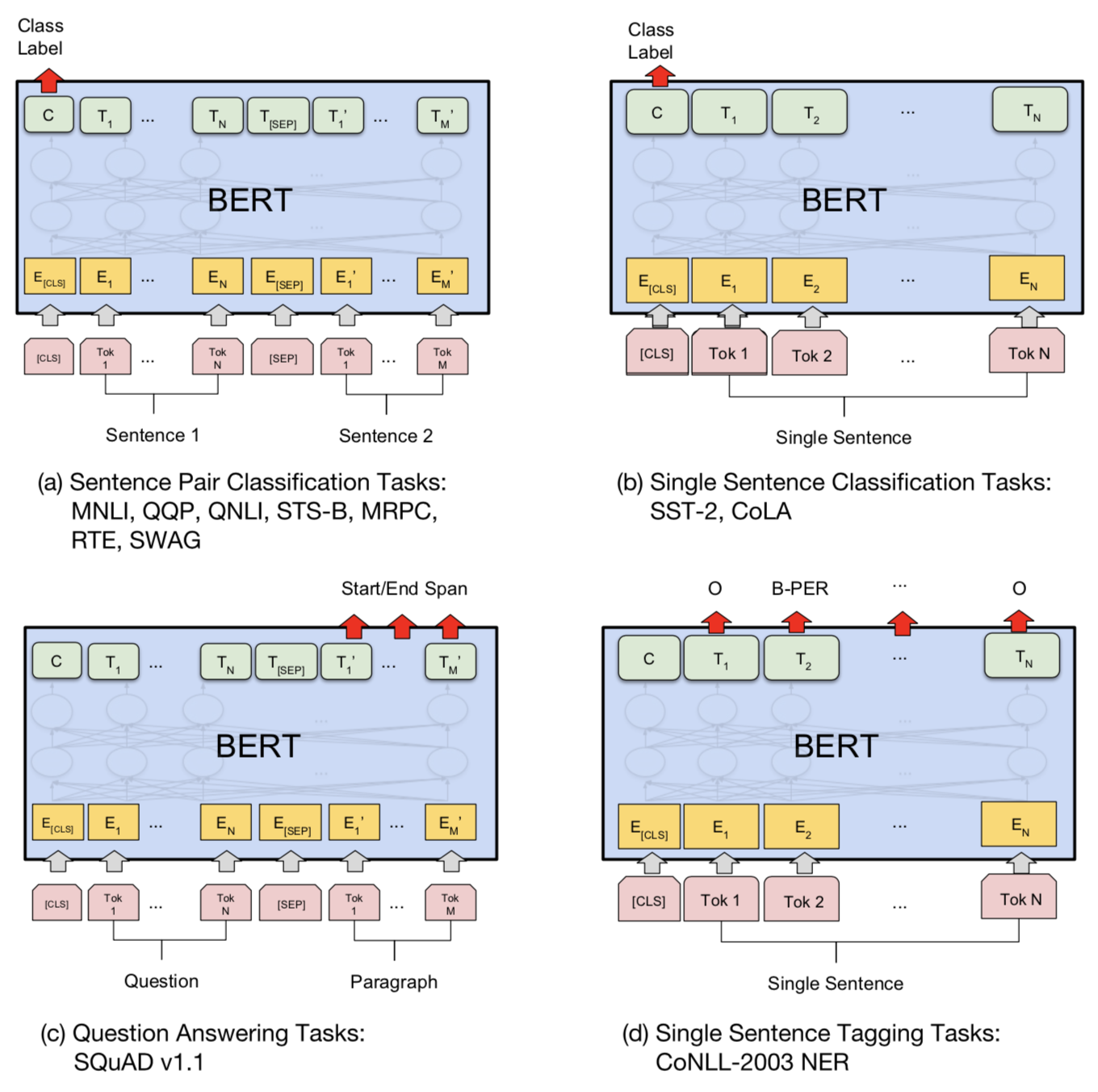
The following summary table highlights differences between fine-tuning OpenAI GPT and BERT.
| | OpenAI GPT | BERT |
| Special char | [SEP] and [CLS] are only introduced at fine-tuning stage. | [SEP] and [CLS] and sentence A/B embeddings are learned at the pre-training stage. |
| Training process | 1M steps, batch size 32k words. | 1M steps, batch size 128k words. |
| Fine-tuning | lr = 5e-5 for all fine-tuning tasks. | Use task-specific lr for fine-tuning. |
ALBERT
ALBERT (Lan, et al. 2019), short for A Lite BERT, is a lightweight variant of the BERT model. Relative to a BERT model with a similar configuration, ALBERT can be trained 1.7x faster and uses 18x fewer parameters. ALBERT introduces three changes: the first two reduce parameter count and memory footprint (and therefore improve training speed), and the third replaces the next sentence prediction (NSP) objective with a more challenging training task.
Factorized Embedding Parameterization
In BERT, the WordPiece embedding size $E$ is set equal to the hidden state size $H$. In other words, if we increase the model size (larger $H$), we must also learn a larger token embedding, which is expensive because it scales with the vocabulary size ($V$).
Conceptually, because token embeddings are intended to capture context-independent representations while hidden states are context-dependent, it is reasonable to decouple the hidden-layer size from the vocabulary embedding size. With factorized embedding parameterization, the large vocabulary embedding matrix of size $V \times H$ is decomposed into two smaller matrices of size $V \times E$ and $E \times H$. For $H \gt E$ or even $H \gg E$, this factorization can substantially reduce parameters.
Cross-layer Parameter Sharing
Cross-layer parameter sharing can be applied in several forms: (a) share only the feed-forward sublayer; (b) share only the attention parameters; or (c) share all parameters. This approach dramatically reduces parameter count while not degrading performance too much.
Sentence-Order Prediction (SOP)
Notably, the next sentence prediction (NSP) task in BERT was found to be too easy. ALBERT instead uses a sentence-order prediction (SOP) self-supervised loss:
- Positive sample: two consecutive segments from the same document.
- Negative sample: the same two segments, but with their order swapped.
For NSP, the model can often succeed by detecting topical differences when A and B come from unrelated contexts. In contrast, SOP is more difficult because it requires modeling coherence and the correct ordering between segments.
GPT-2
The OpenAI GPT-2 language model is a direct successor to GPT. GPT-2 has 1.5B parameters, 10x more than the original GPT, and it achieves state-of-the-art results on 7 of 8 evaluated language modeling datasets in a zero-shot transfer setting without task-specific fine-tuning. Its pre-training dataset contains 8 million web pages collected by crawling qualified outbound links from Reddit. Improvements from GPT-2 are particularly noticeable on small datasets and on datasets designed to measure long-term dependency.
Zero-Shot Transfer
GPT-2 is pre-trained solely with the language modeling objective. Downstream language tasks are formulated in terms of conditional probability prediction, and no task-specific fine-tuning is performed.
- Text generation follows directly from language modeling.
- Machine translation, for example from English to Chinese, can be induced by conditioning the language model on example pairs of “English sentence = Chinese sentence” and appending “the target English sentence =” at the end.
- For example, a conditional probability to predict might look like:
P(? | I like green apples. = 我喜欢绿苹果。 A cat meows at him. = 一只猫对他喵。It is raining cats and dogs. =")
- For example, a conditional probability to predict might look like:
- QA can be formatted similarly to translation by providing question and answer pairs in the context.
- Summarization can be induced by appending
TL;DR:after the article text in the context.
BPE on Byte Sequences
Like the original GPT, GPT-2 uses BPE, but it applies BPE to UTF-8 byte sequences. Each byte represents 256 possible values in 8 bits, while UTF-8 can use up to 4 bytes per character, supporting up to $2^{31}$ characters in total. As a result, byte-level representation requires only a 256-item vocabulary and removes the need for preprocessing steps such as tokenization. Despite these benefits, current byte-level language models still exhibit a non-negligible performance gap relative to state-of-the-art word-level models.
BPE greedily merges frequently co-occurring byte pairs. To avoid producing multiple variants of common words (for example, dog., dog!, and dog? for dog), GPT-2 prevents BPE merges across character categories (so dog is not merged with punctuation such as ., !, or ?). This trick helps improve the quality of the resulting byte segmentation.
With byte sequence representation, GPT-2 can assign a probability to any Unicode string, independent of preprocessing choices.
Model Modifications
Beyond increasing the number of Transformer layers and parameters, GPT-2 introduces only a small set of architectural modifications relative to GPT:
- Layer normalization was moved to the input of each sub-block, analogous to a residual unit of type “building block” (unlike the original “bottleneck” type, which applies batch normalization before weight layers).
- An additional layer normalization was added after the final self-attention block.
- A modified initialization was defined as a function of model depth.
- The residual layer weights were initially scaled by a factor of $1/ \sqrt{N}$, where N is the number of residual layers.
- A larger vocabulary size and context size were used.
RoBERTa
RoBERTa (short for Robustly optimized BERT approach; Liu, et al. 2019) presents a revised recipe for training BERT to obtain stronger results, motivated by the finding that the original BERT model was significantly undertrained. The recipe includes the following observations:
- Train longer and use a larger batch size.
- Remove the next sentence prediction (NSP) task.
- Use longer sequences in the training data format. The paper reports that using individual sentences as inputs harms downstream performance; instead, multiple contiguous sentences should be sampled to form longer segments.
- Use dynamic masking patterns. In the original BERT, masking is applied once during preprocessing, producing a static mask across epochs. RoBERTa applies masking in 10 different ways across 40 epochs.
RoBERTa also adds the CommonCrawl News dataset and further supports the conclusion that pretraining with more data helps improve downstream performance. It is trained using BPE on byte sequences, the same approach used in GPT-2. The work also emphasizes that hyperparameter choices can significantly affect model performance.
T5
T5 is short for Text-to-Text Transfer Transformer (Raffel et al., 2020). Its encoder-decoder implementation follows the original Transformer design: tokens → embedding → encoder → decoder → output. T5 adopts the “Natural Language Decathlon” framework (McCann et al., 2018), which maps many standard NLP tasks into question answering over a context. Rather than using an explicit QA format, T5 uses short task prefixes to indicate the task intent and fine-tunes the model separately for each task. This text-to-text framing simplifies transfer learning evaluation by enabling the same model to be applied across a broad range of tasks.
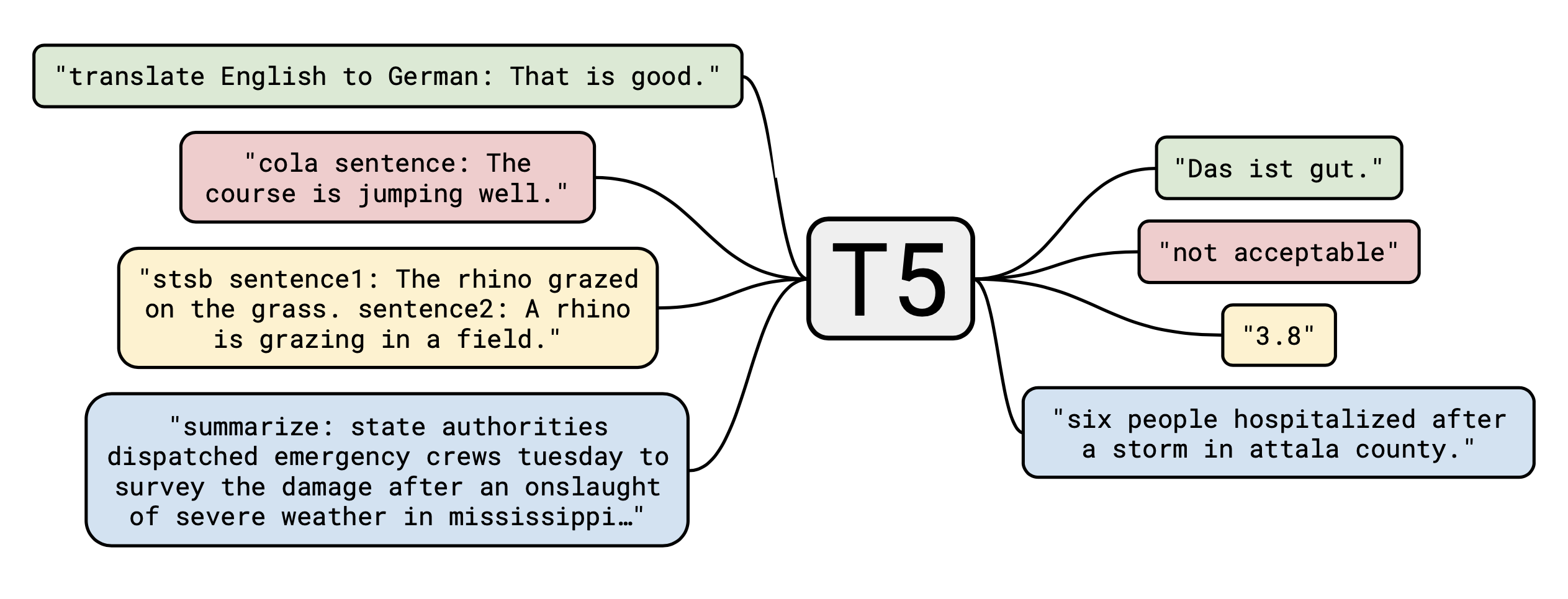
The model is trained on a web corpus extracted in April 2019 with multiple filters applied. For each downstream task, it is fine-tuned separately using either “adapter layers” (adding an extra layer for training) or “gradual unfreezing” (see ULMFiT). Both approaches update only a subset of parameters while leaving most model parameters unchanged. T5-11B achieved state-of-the-art results on many NLP tasks.
As the authors note, “…our goal is not to propose new methods but instead to provide a comprehensive perspective on where the field stands”. The long T5 paper details training configurations and evaluation procedures extensively, and it is a useful read for anyone interested in training a language model from scratch.
GPT-3
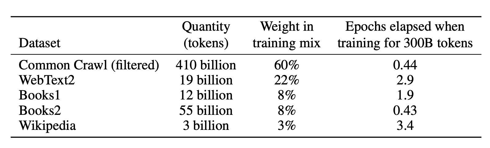
GPT-3 (Brown et al., 2020) uses the same architecture as GPT-2 but scales to 175B parameters, which is 10x larger than GPT-2 (1.5B). In addition, GPT-3 uses alternating dense and locally banded sparse attention patterns, as in the sparse transformer. To fit a model of this size across multiple GPUs, training partitions are applied along both the width and depth dimensions. The training data is a filtered version of Common Crawl combined with several other high-quality curated datasets. To reduce contamination from downstream benchmarks appearing in the training data, the authors attempted to remove all overlaps with the benchmark datasets under study. However, the filtering process was not fully successful due to a bug.
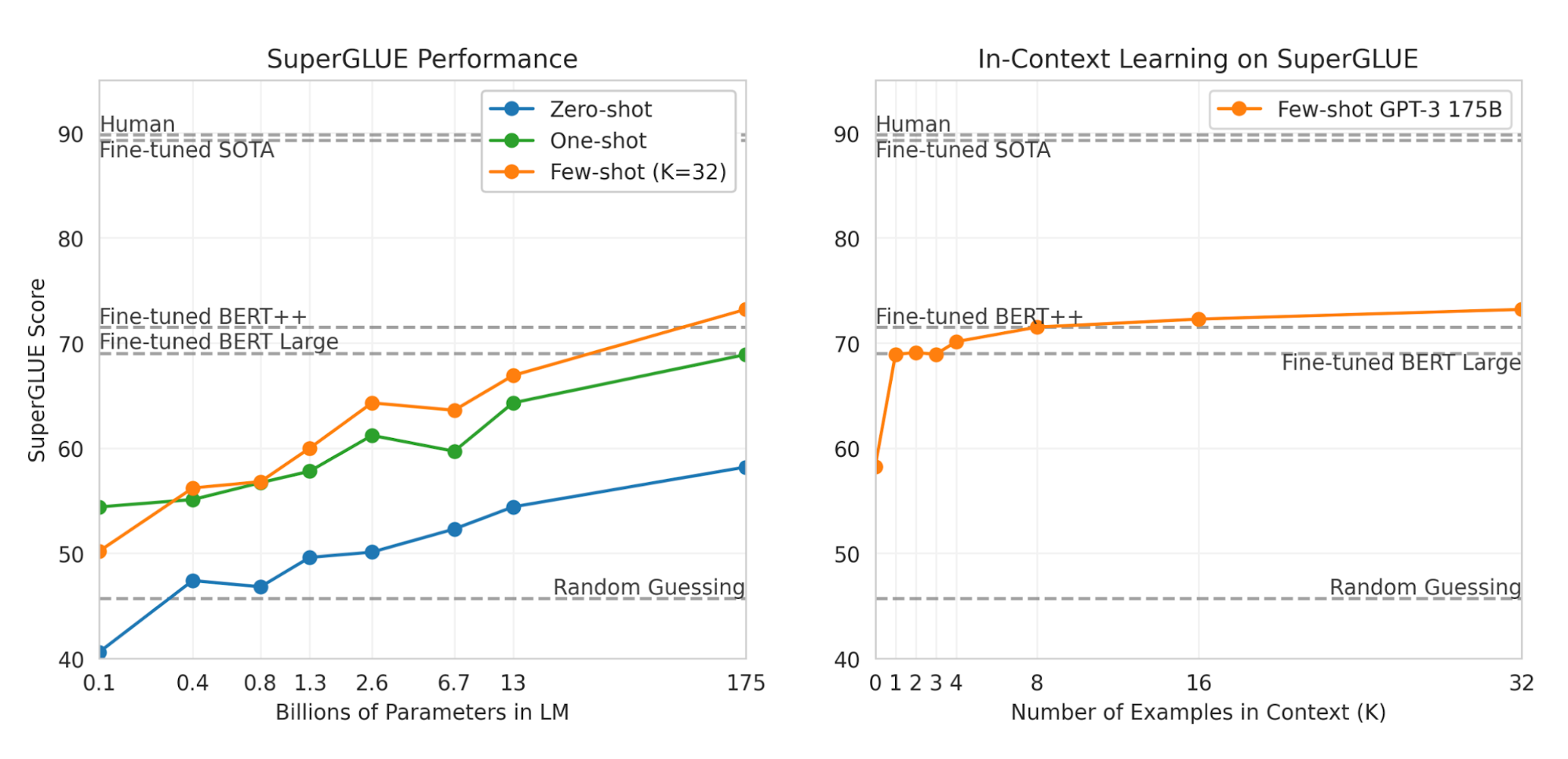
For downstream evaluation, GPT-3 is tested in a few-shot setting without gradient-based fine-tuning. In this setup, the few-shot examples are included directly in the prompt. GPT-3 achieves strong results on many NLP datasets, comparable to fine-tuned BERT models.
XLNet
Autoregressive (AR) models such as GPT and autoencoder (AE) models such as BERT are two common approaches to language modeling. However, each has drawbacks: AR models do not learn bidirectional context, which is important for downstream tasks such as reading comprehension, while AE models assume masked positions are independent given all other unmasked tokens, which oversimplifies long-range dependencies.
XLNet (Yang et al. 2019) generalizes the AE approach to incorporate the benefits of AR. XLNet proposes the permutation language modeling objective. Given a text sequence, it samples a factorization order $\mathbf{z}$ and decomposes the likelihood $p_\theta(\mathbf{x})$ according to that factorization order,
where $\mathcal{Z}_T$ is the set of all possible permutations of length $T$; $z_t$ and $\mathbf{z}_{
Note that the naive representation of the hidden state of the context, $h_\theta (\mathbf{x}_{\mathbf{z}_{
However, two different requirements on $g_\theta (\mathbf{x}_{\mathbf{z}_{
- When predicting $x_{z_t}$, the representation should encode only the position $z_t$ and not the content $x_{z_t}$; otherwise the task becomes trivial. This is captured by the “query representation” $g_{z_t} = g_\theta (\mathbf{x}_{\mathbf{z}_{
- When predicting $x_j$ where $j > t$, the representation should also encode the content $x_{z_t}$ to provide full context. This is the “content representation” $h_{z_t} = h_\theta(\mathbf{x}_{\leq t})$.
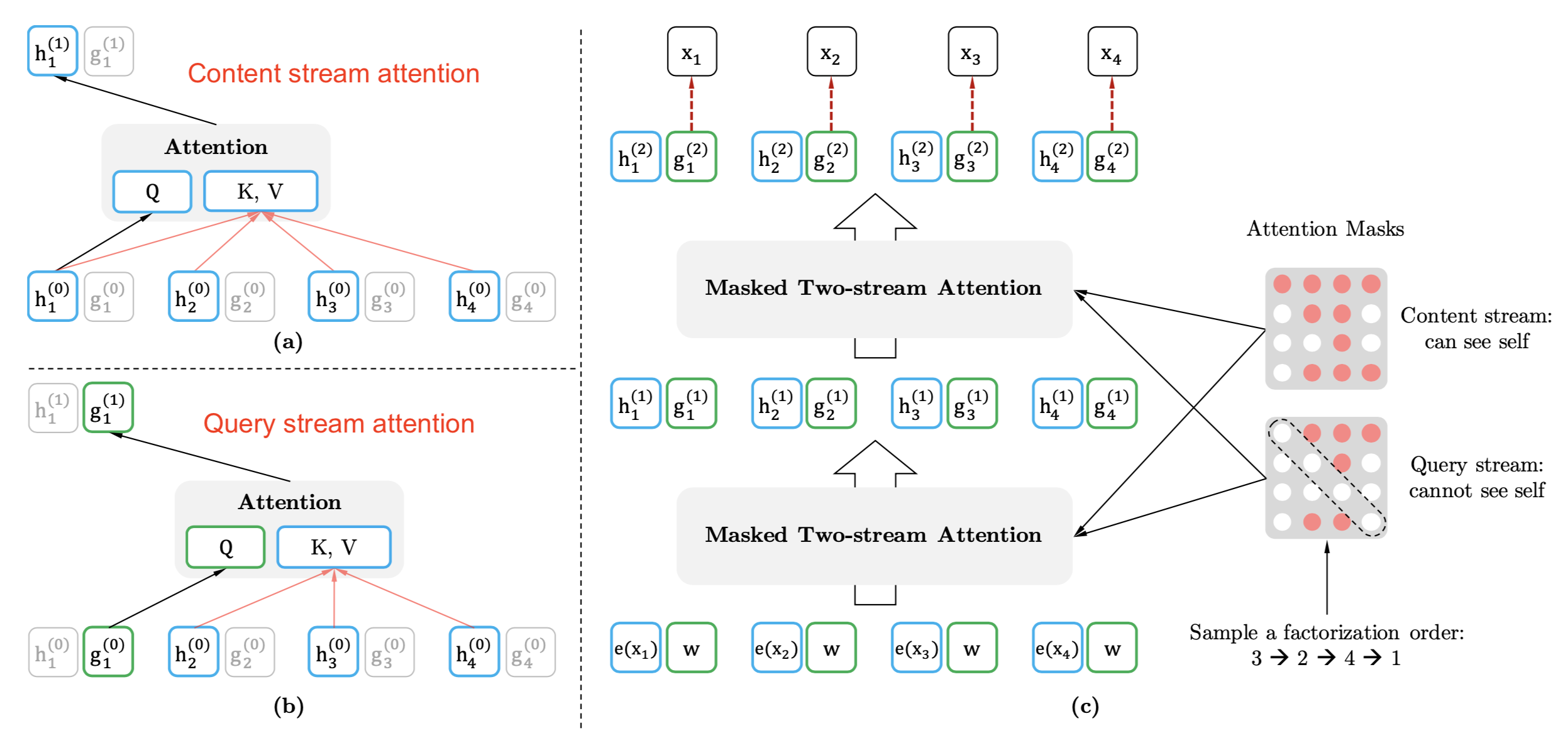
Conceptually, the two representation streams are updated as follows:
Because permutation language modeling is difficult to optimize, XLNet is configured to predict only the last chunk of tokens under a given factorization order.
The “XL” in XLNet is derived from Transformer-XL. XLNet incorporates Transformer-XL’s mechanism for extending attention span by reusing hidden states from earlier segments.

BART
BART (Lewis et al., 2019) is a denoising autoencoder trained to recover original text from a randomly corrupted version. It combines Bidirectional and AutoRegressive Transformer by jointly training a BERT-like bidirectional encoder with a GPT-like autoregressive decoder. The loss is simply to minimize the negative log-likelihood.
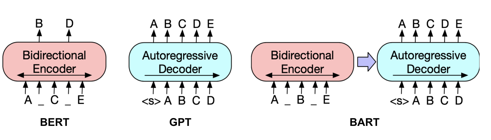
The authors evaluated a range of noising transformations, including token masking, token deletion, text infilling (that is, a randomly sampled span, potentially containing multiple tokens, is replaced with a single [MASK] token), sentence permutation, and documentation rotation (that is, a document is rotated to begin at a random token). The best-performing noising strategy they identified combines text infilling with sentence shuffling.
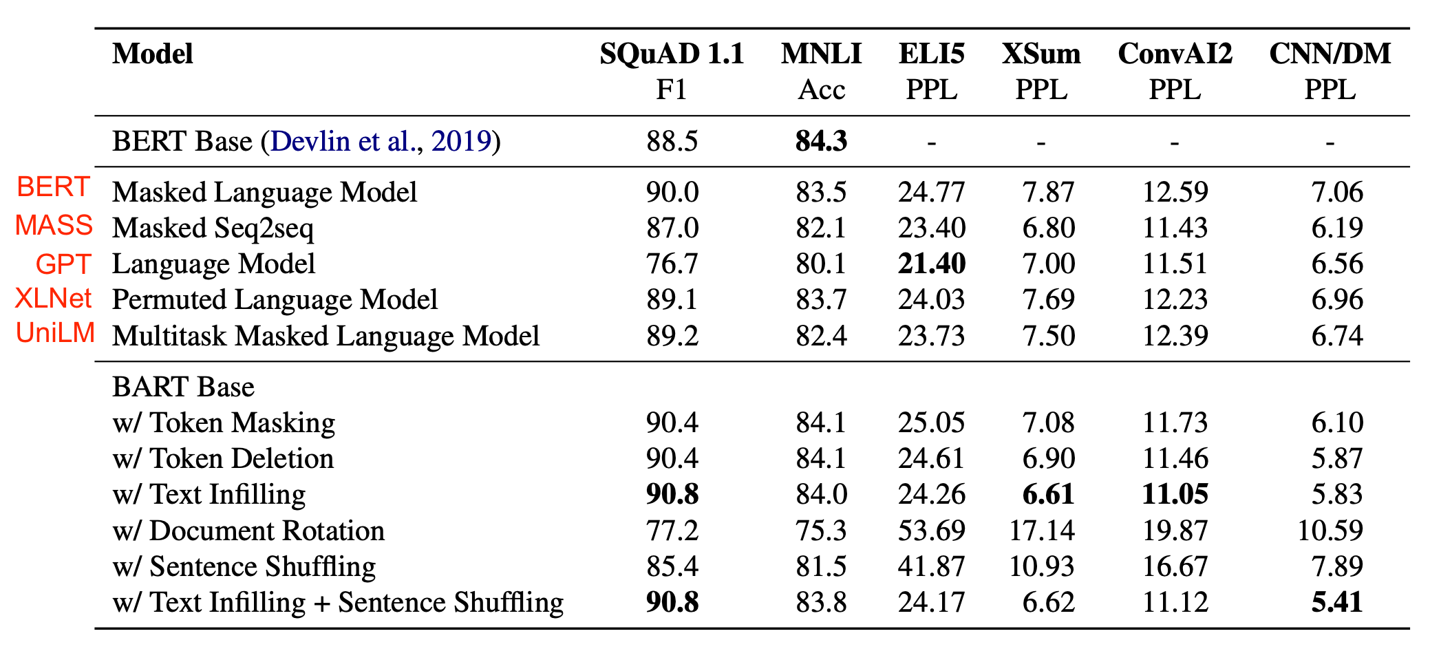
Key takeaways from their experiments:
- Pre-training methods vary substantially in effectiveness across downstream tasks.
- Token masking is essential, performance is poor when using only sentence permutation or documentation rotation.
- Left-to-right pre-training improves generation.
- Bidirectional encoders are essential for SQuAD.
- The pre-training objective is not the only critical factor; architectural improvements such as relative-position embeddings or segment-level recurrence also matter.
- Autoregressive language models perform best on ELI5.
- BART delivers the most consistently strong overall performance.
ELECTRA
Many large pre-trained language models require substantial computational resources, which raises concerns about cost and accessibility. ELECTRA (“Efficiently Learning an Encoder that Classifies Token Replacements Accurately”; Clark et al. 2020) targets improved pre-training efficiency by reframing language modeling as a discrimination task rather than a generation task.
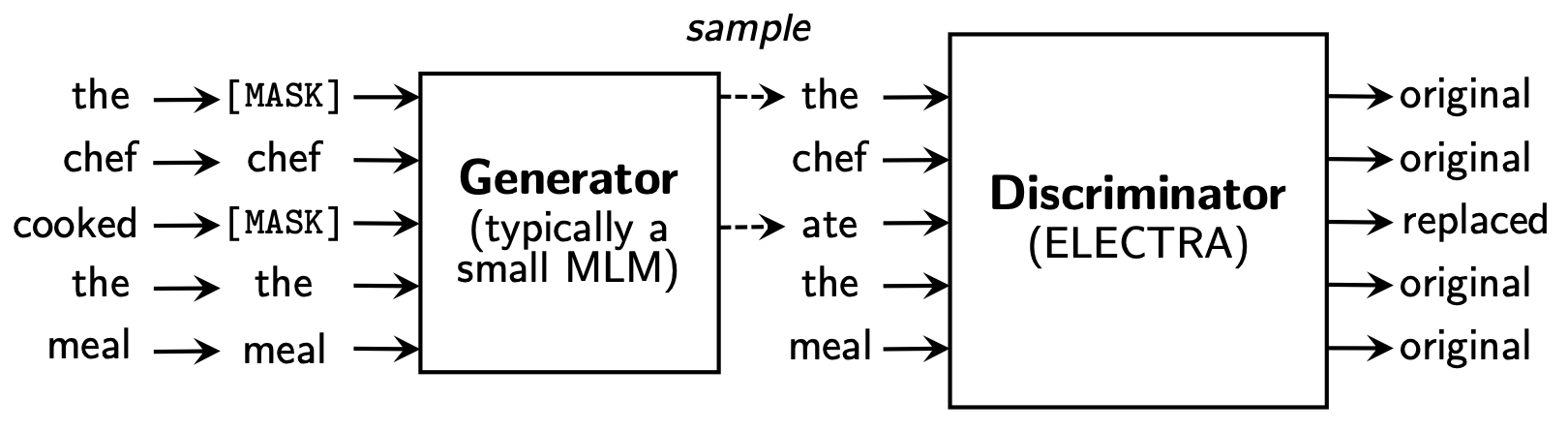
ELECTRA introduces a pre-training task called Replaced Token Detection (RTD). First, randomly sample $k$ positions to mask. Each selected token in the original text is replaced by a plausible alternative predicted by a small language model, the generator $G$. Then the discriminator $D$ predicts, for each token, whether it is original or replaced.
The generator loss is negative log-likelihood, as in other language models. The discriminator loss is cross-entropy. Note that the generator is not adversarially trained to fool the discriminator, it is trained only to optimize NLL, since experiments showed negative results for adversarial training.
The authors found it more effective to share only the embeddings between the generator and discriminator while keeping the generator small (about 1/4 to 1/2 of the discriminator size), rather than sharing all weights (which would force the two models to have identical size). They also report that jointly training the generator and discriminator performs better than a two-stage approach that alternates training each model.
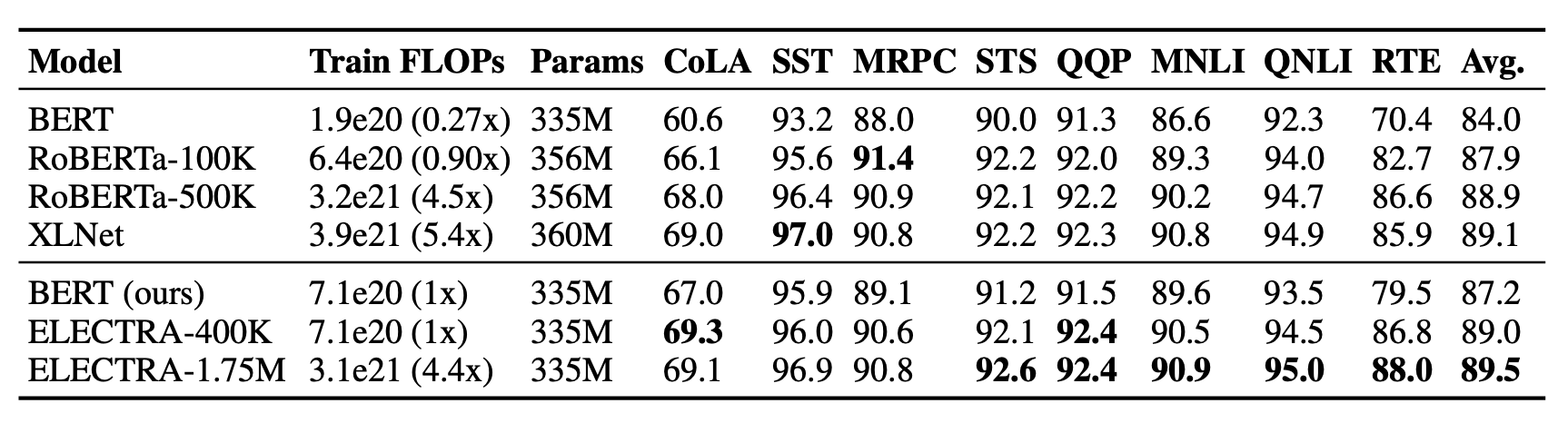
After pre-training, the generator is discarded, and only the ELECTRA discriminator is fine-tuned for downstream tasks. The following table reports ELECTRA’s performance on the GLUE dev set.
Summary
| Base model | Pretraining Tasks | |
|---|---|---|
| CoVe | seq2seq NMT model | supervised learning using translation dataset. |
| ELMo | two-layer biLSTM | next token prediction |
| CVT | two-layer biLSTM | semi-supervised learning using both labeled and unlabeled datasets |
| ULMFiT | AWD-LSTM | autoregressive pretraining on Wikitext-103 |
| GPT | Transformer decoder | next token prediction |
| BERT | Transformer encoder | mask language model + next sentence prediction |
| ALBERT | same as BERT but light-weighted | mask language model + sentence order prediction |
| GPT-2 | Transformer decoder | next token prediction |
| RoBERTa | same as BERT | mask language model (dynamic masking) |
| T5 | Transformer encoder + decoder | pre-trained on a multi-task mixture of unsupervised and supervised tasks and for which each task is converted into a text-to-text format. |
| GPT-3 | Transformer decoder | next token prediction |
| XLNet | same as BERT | permutation language modeling |
| BART | BERT encoder + GPT decoder | reconstruct text from a noised version |
| ELECTRA | same as BERT | replace token detection |
Metric: Perplexity
Perplexity is commonly used as an intrinsic evaluation metric to assess how well a language model captures the true word distribution conditioned on context.
The perplexity of a discrete probability distribution $p$ is defined as the exponential of its entropy:
Given a sentence with $N$ words, $s = (w_1, \dots, w_N)$, the entropy can be written as follows, under the simplifying assumption that each word has the same frequency, $\frac{1}{N}$:
The perplexity for the sentence is then:
A strong language model should assign high probability to the correct words. Therefore, lower perplexity is better.
Common Tasks and Datasets
- SQuAD (Stanford Question Answering Dataset): A reading comprehension dataset consisting of questions over Wikipedia articles, where each answer is a span of text.
- RACE (ReAding Comprehension from Examinations): A large-scale reading comprehension dataset with more than 28,000 passages and nearly 100,000 questions. It is collected from English examinations in China designed for middle school and high school students.
- See more QA datasets in a later post.
Commonsense Reasoning
- Story Cloze Test: A commonsense reasoning framework for evaluating story understanding and generation. The test requires a system to choose the correct ending to multi-sentence stories from two options.
- SWAG (Situations With Adversarial Generations): multiple choices; contains 113k sentence-pair completion examples that evaluate grounded common-sense inference
Natural Language Inference (NLI): also known as Text Entailment, a task that determines, in logic, whether one sentence can be inferred from another.
- RTE (Recognizing Textual Entailment): A set of datasets initiated by textual entailment challenges.
- SNLI (Stanford Natural Language Inference): A collection of 570k human-written English sentence pairs manually labeled for balanced classification with labels
entailment,contradiction, andneutral. - MNLI (Multi-Genre NLI): Similar to SNLI, but covering a wider range of writing styles and topics, collected from transcribed speech, popular fiction, and government reports.
- QNLI (Question NLI): Converted from SQuAD into a binary classification task over (question, sentence) pairs.
- SciTail: An entailment dataset created from multiple-choice science exams and web sentences.
Named Entity Recognition (NER): labels sequences of words in text that correspond to names of entities such as people and companies, or gene and protein names
- CoNLL 2003 NER task: consists of Reuters newswire, focusing on four named entity types: persons, locations, organizations, and miscellaneous entities.
- OntoNotes 5.0: This corpus contains English, Arabic, and Chinese text, tagged with four entity types (PER, LOC, ORG, MISC).
- Reuters Corpus: A large collection of Reuters news stories.
- Fine-Grained NER (FGN)
Sentiment Analysis
- SST (Stanford Sentiment Treebank)
- IMDb: A large dataset of movie reviews with binary sentiment classification labels.
Semantic Role Labeling (SRL): models the predicate-argument structure of a sentence, and is often described as answering “Who did what to whom”.
Sentence similarity: also known as paraphrase detection
- MRPC (MicRosoft Paraphrase Corpus): Contains sentence pairs extracted from news sources on the web, annotated to indicate whether each pair is semantically equivalent.
- QQP (Quora Question Pairs) STS Benchmark: Semantic Textual Similarity
Sentence Acceptability: a task that labels sentences for grammatical acceptability.
- CoLA (Corpus of Linguistic Acceptability): a binary single-sentence classification task.
Text Chunking: dividing text into syntactically correlated word groups.
Part-of-Speech (POS) Tagging: assigns a part of speech to each token, such as noun, verb, or adjective. the Wall Street Journal portion of the Penn Treebank (Marcus et al., 1993).
Machine Translation: See the Standard NLP page.
- WMT 2015 English-Czech data (Large)
- WMT 2014 English-German data (Medium)
- IWSLT 2015 English-Vietnamese data (Small)
Coreference Resolution: clusters mentions in text that refer to the same underlying real-world entities.
Long-range Dependency
- LAMBADA (LAnguage Modeling Broadened to Account for Discourse Aspects): A collection of narrative passages extracted from BookCorpus; the task is to predict the last word, requiring at least 50 tokens of context for a human to succeed.
- Children’s Book Test: built from books that are freely available in Project Gutenberg. The task is to predict a missing word among 10 candidates.
Multi-task benchmark
- GLUE multi-task benchmark: https://gluebenchmark.com
- decaNLP benmark: https://decanlp.com
Unsupervised pretraining dataset
- Books corpus: The corpus contains “over 7,000 unique unpublished books from a variety of genres including Adventure, Fantasy, and Romance.”
- 1B Word Language Model Benchmark
- English Wikipedia: ~2500M words
Cited as:
@article{weng2019LM,
  title   = "Generalized Language Models",
  author  = "Weng, Lilian",
  journal = "lilianweng.github.io",
  year    = "2019",
  url     = "https://lilianweng.github.io/posts/2019-01-31-lm/"
}
Reference
[1] Bryan McCann, et al. “Learned in translation: Contextualized word vectors.” NIPS. 2017.
[2] Kevin Clark et al. “Semi-Supervised Sequence Modeling with Cross-View Training.” EMNLP 2018.
[3] Matthew E. Peters, et al. “Deep contextualized word representations.” NAACL-HLT 2017.
[4] OpenAI Blog “Improving Language Understanding with Unsupervised Learning”, June 11, 2018.
[5] OpenAI Blog “Better Language Models and Their Implications.” Feb 14, 2019.
[6] Jeremy Howard and Sebastian Ruder. “Universal language model fine-tuning for text classification.” ACL 2018.
[7] Alec Radford et al. “Improving Language Understanding by Generative Pre-Training”. OpenAI Blog, June 11, 2018.
[8] Jacob Devlin, et al. “BERT: Pre-training of deep bidirectional transformers for language understanding.” arXiv:1810.04805 (2018).
[9] Mike Schuster, and Kaisuke Nakajima. “Japanese and Korean voice search.” ICASSP. 2012.
[10] Google’s Neural Machine Translation System: Bridging the Gap between Human and Machine Translation
[11] Ashish Vaswani, et al. “Attention is all you need.” NIPS 2017.
[12] Peter J. Liu, et al. “Generating wikipedia by summarizing long sequences.” ICLR 2018.
[13] Sebastian Ruder. “10 Exciting Ideas of 2018 in NLP” Dec 2018.
[14] Alec Radford, et al. “Language Models are Unsupervised Multitask Learners.”. 2019.
[15] Rico Sennrich, et al. “Neural machine translation of rare words with subword units.” arXiv preprint arXiv:1508.07909. 2015.
[16] Zhenzhong Lan, et al. “ALBERT: A Lite BERT for Self-supervised Learning of Language Representations.” arXiv Preprint arXiv:1909.11942 (2019).
[17] Yinhan Liu, et al. “RoBERTa: A Robustly Optimized BERT Pretraining Approach.” arXiv Preprint arXiv:1907.11692 (2019).
[18] Tom B Brown, et al. “Language Models are Few-Shot Learners” NeuriPS 2020.
[19] Zhilin Yang et al. “XLNet: Generalized Autoregressive Pretraining for Language Understanding.” NeuriPS 2019.
[20] Mike Lewis et al. “BART: Denoising Sequence-to-Sequence Pre-training for Natural Language Generation, Translation, and Comprehension.” ACL 2020.
[21] Kevin Clark et al. “ELECTRA: Pre-training Text Encoders as Discriminators Rather Than Generators.” ICLR 2020.
[22] Colin Raffel, et al. “Exploring the Limits of Transfer Learning with a Unified Text-to-Text Transformer” JMLR 2020.