Robotics

Domain Randomization for Sim2Real Transfer

In robotics, one of the most challenging problems is enabling a model trained in simulation to transfer reliably to the real world. Because deep reinforcement learning (RL) algorithms are sample-inefficient and collecting data on real robots is expensive, models often must be trained in a simulator, which in principle can generate an unlimited amount of data. In practice, however, the reality gap between simulation and the physical world frequently causes failures during deployment on real hardware. This gap is driven by mismatches in physical parameters (for example, friction, kp, damping, mass, density) and, more critically, by inaccurate physical modeling (for example, collisions involving soft surfaces).

2019 · 14 min read · Curated and presented by Arthur Sedek

If a model or policy is trained primarily in a simulator but is ultimately expected to operate on a physical robot, it will almost certainly encounter the sim2real gap. Domain Randomization (DR) is a straightforward yet highly effective approach for narrowing this gap by randomizing properties of the training environment.

In robotics, one of the most challenging problems is enabling a model to transfer reliably to the real world. Because deep RL algorithms are sample-inefficient and collecting data on real robots is costly, we frequently train models in simulation, where, in principle, we can obtain an unlimited amount of data. In practice, however, differences between the simulator and the physical world often cause models to fail once deployed on real robots. This gap is driven by mismatched physical parameters (for example, friction, kp, damping, mass, density) and, more critically, by incorrect physical modeling (for example, collisions involving soft surfaces).

To reduce the sim2real gap, one option is to improve the simulator so that it more closely matches reality. Several approaches are commonly used:

System identification
- System identification builds a mathematical model of a physical system. In the RL setting, this mathematical model is the simulator. Making the simulator more realistic therefore requires careful calibration.
- Unfortunately, calibration is expensive. In addition, many physical parameters for the same machine can vary substantially due to temperature, humidity, positioning, or wear and tear over time.
Domain adaptation
- Domain adaptation (DA) refers to a family of transfer learning methods that update the simulated data distribution to match the real distribution, typically via a mapping or a regularization term enforced by the task model.
- Many DA models, especially those used for image classification or end-to-end image-based RL tasks, are built around adversarial losses or GAN.
Domain randomization
- With domain randomization (DR), we create many simulated environments whose properties are randomized, and then train a model that performs well across all of them.
- This model is likely to adapt to the real-world environment, since the real system is expected to be one sample from the rich distribution of variations seen during training.

Both DA and DR are unsupervised. Compared with DA, which typically needs a reasonable quantity of real samples to capture the real distribution, DR may require only a little or no real data. DR is the focus of this post.

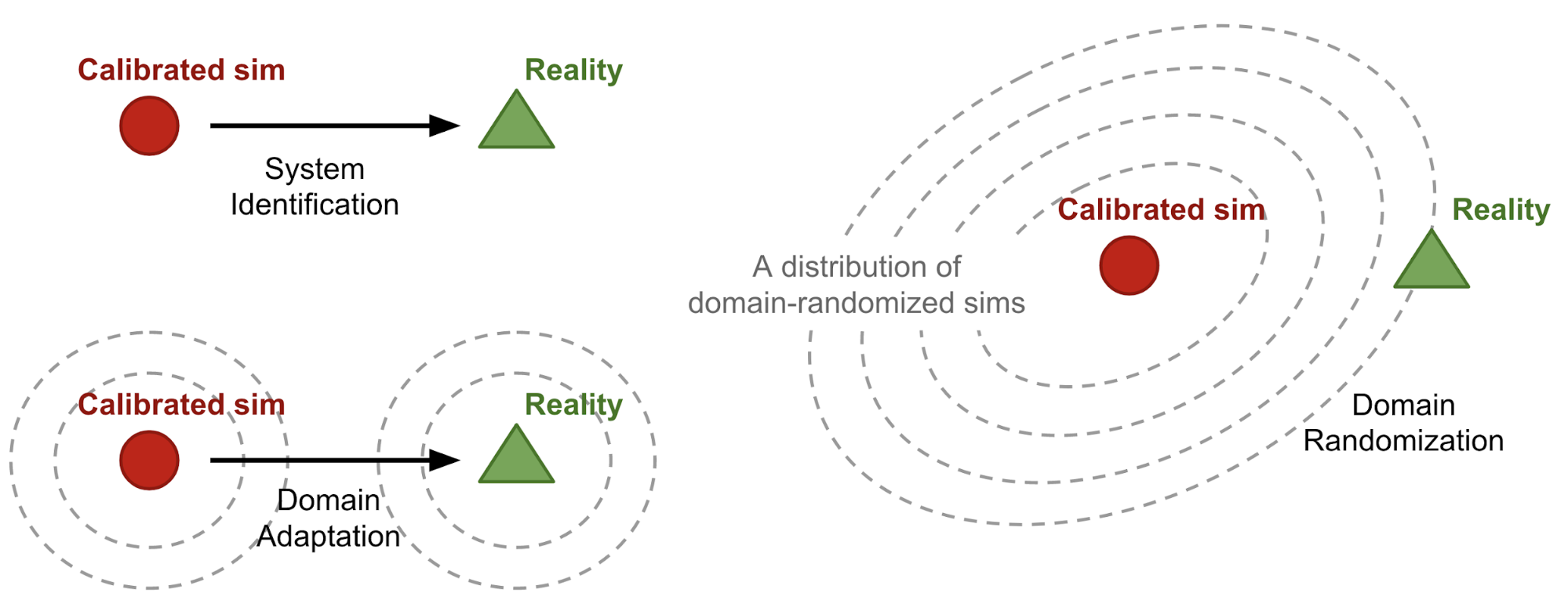
Conceptual illustrations of three approaches for sim2real transfer.

What is Domain Randomization?

To express the definition in more general terms, we call the environment to which we have full access (that is, the simulator) the source domain, and the environment to which we want to transfer the model the target domain (that is, the physical world). Training occurs in the source domain. In the source domain $e_\xi$, we can control a set of $N$ randomization parameters using a configuration $\xi$, sampled from a randomization space, $\xi \in \Xi \subset \mathbb{R}^N$.

During policy training, episodes are collected in the source domain with randomization applied. As a result, the policy experiences a wide variety of environments and learns to generalize. The policy parameter $\theta$ is trained to maximize the expected reward $R(.)$, averaged over a distribution of configurations:

$ \theta^* = \arg\max_\theta \mathbb{E}_{\xi \sim \Xi} [\mathbb{E}_{\pi_\theta, \tau \sim e_\xi} [R(\tau)]] $

where $\tau_\xi$ is a trajectory collected in the source domain after randomization with $\xi$. Put differently, “discrepancies between the source and target domains are modeled as variability in the source domain.” (quote from Peng et al. 2018).

Uniform Domain Randomization

In the original formulation of DR (Tobin et al, 2017; Sadeghi et al. 2016), each randomization parameter $\xi_i$ is bounded by an interval $\xi_i \in [\xi_i^\text{low}, \xi_i^\text{high}], i=1,\dots,N$, and each parameter is sampled uniformly within that range.

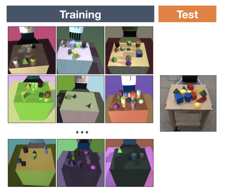
Randomization parameters can control the visual appearance of the scene, including, but not limited to, the following (see Fig. 2). A model trained on simulated images with such randomization can transfer to real, non-randomized images.

Object position, shape, and color,
Material texture,
Lighting conditions,
Random noise injected into images,
Camera position, orientation, and field of view in the simulator.

Images captured in the training environment are randomized. (Image source: Tobin et al, 2017)

It is also possible to randomize physical dynamics within the simulator (Peng et al. 2018). Prior work has shown that a recurrent policy can adapt to different physical dynamics, including partially observable aspects of reality. Randomized physical dynamics features include, but are not limited to:

Object mass and dimensions,
Robot body mass and dimensions,
Joint damping, kp, and friction,
PID controller gains (P term),
Joint limits,
Action delay,
Observation noise.

At OpenAI Robotics, combining visual DR with dynamics DR enabled us to learn a policy that runs on a real dexterous robot hand (OpenAI, 2018). The manipulation task trains the robot hand to rotate an object continuously so it can achieve 50 successive random target orientations. The sim2real gap for this task is substantial due to (a) the large number of simultaneous contacts between the robot and the object and (b) imperfect simulation of object collisions and other motions. Initially, the policy could barely last more than 5 seconds before dropping the object. With DR, however, the policy eventually improved and performed surprisingly well in reality.

Why does Domain Randomization Work?

This raises a natural question: why does domain randomization work so well? Although the core idea is simple, two non-exclusive explanations are particularly compelling.

DR as Optimization

One perspective (Vuong, et al, 2019) is to treat the choice of randomization parameters in DR as a bilevel optimization problem. If we assume access to the real environment $e_\text{real}$ and that the randomization configuration is sampled from a distribution parameterized by $\phi$, $\xi \sim P_\phi(\xi)$, then the goal is to learn a distribution such that a policy $\pi_\theta$ trained under it achieves maximal performance in $e_\text{real}$:

$ \begin{aligned} &\phi^* = \arg\min_{\phi} \mathcal{L}(\pi_{\theta^*(\phi)}; e_\text{real}) \\ \text{where } &\theta^*(\phi) = \arg\min_\theta \mathbb{E}_{\xi \sim P_\phi(\xi)}[\mathcal{L}(\pi_\theta; e_\xi)] \end{aligned} $

where $\mathcal{L}(\pi; e)$ is the loss function of policy $\pi$ evaluated in environment $e$.

Although uniform DR uses hand-selected randomization ranges, in practice this often depends on domain expertise and multiple rounds of trial-and-error adjustments guided by transfer performance. In effect, this becomes a manual optimization process in which $\phi$ is tuned to obtain the best $\mathcal{L}(\pi_{\theta^*(\phi)}; e_\text{real})$.

The guided domain randomization methods discussed next are heavily influenced by this viewpoint, with the aim of performing bilevel optimization and automatically learning the most effective parameter distribution.

DR as Meta-Learning

In our dexterity learning project (OpenAI, 2018), we trained an LSTM policy to generalize across varying environment dynamics. We observed that after the robot completed the first rotation, the time required for subsequent successes decreased substantially. We also found that a feedforward (FF) policy without memory was unable to transfer to a physical robot. Together, these observations suggest that the policy is learning and adapting online to a new environment.

In this sense, domain randomization effectively constructs a collection of different tasks. Memory in the recurrent network allows the policy to perform meta-learning across tasks, and then succeed in a real-world setting.

Guided Domain Randomization

Vanilla DR assumes no access to real data. It therefore samples randomization configurations as broadly and uniformly as possible in simulation, with the hope that the real environment is contained within that wide distribution. It is natural to consider more sophisticated strategies, replacing uniform sampling with guidance from task performance, real data, or the simulator.

One motivation for guided DR is to reduce computation by avoiding training in unrealistic environments. Another is to prevent infeasible solutions that may arise from overly broad randomization distributions and that can make policy learning difficult.

Optimization for Task Performance

Suppose we train a family of policies using different randomization parameters $\xi \sim P_\phi(\xi)$, where $P_\xi$ is the distribution for $\xi$ parameterized by $\phi$. We then evaluate each one on the downstream task in the target domain (for example, controlling a robot in the real world or evaluating on a validation set) and collect feedback. This feedback indicates how effective a configuration $\xi$ is, and it provides the signal needed to optimize $\phi$.

Motivated by NAS, AutoAugment (Cubuk, et al. 2018) formulates the problem of learning the best data augmentation operations (for example, shearing, rotation, inversion) for image classification as an RL problem. Although AutoAugment was not proposed specifically for sim2real transfer, it fits within the category of DR guided by task performance. Each augmentation configuration is evaluated on an evaluation set, and the performance improvement is used as a reward to train a PPO policy. This policy produces distinct augmentation strategies for different datasets. For example, for CIFAR-10, AutoAugment tends to select color-based transformations, while ImageNet tends to favor geometric ones.

Ruiz (2019) treated task feedback as an RL reward and proposed an RL-based method, “learning to simulate,” for adjusting $\xi$. A policy is trained to predict $\xi$, using performance metrics on the validation data of the main task as rewards, and the distribution is modeled as a multivariate Gaussian. The overall approach is similar to AutoAugment, applying NAS-like ideas to data generation. Their experiments suggest that even if the main task model has not converged, it can still provide a useful signal for the data generation policy.

An overview of the "learning to simulate" approach. (Image source: Ruiz (2019))

Evolutionary algorithms provide another option, where feedback is treated as fitness to guide evolution (Yu et al, 2019). In this study, they used CMA-ES (covariance matrix adaptation evolution strategy). Fitness is defined as the target-environment performance of a $\xi$-conditional policy. In the appendix, they compare CMA-ES with alternative ways of modeling the dynamics of $\xi$, including Bayesian optimization and neural networks. Their main claim is that those alternatives are less stable or sample-efficient than CMA-ES. Interestingly, when modeling $P(\xi)$ with a neural network, an LSTM is reported to significantly outperform an FF model.

Some argue that the sim2real gap comprises both an appearance gap and a content gap, and that many GAN-inspired DA models focus mainly on the appearance gap. Meta-Sim (Kar, et al. 2019) targets the content gap by generating task-specific synthetic datasets. Meta-Sim uses self-driving car training as an example, where scenes can be highly complex. In this setting, synthetic scenes are parameterized by a hierarchy of objects with properties (for example, location, color) as well as relationships between objects. The hierarchy is specified by a probabilistic scene grammar similar to structured domain randomization (SDR; Prakash et al., 2018), and it is assumed to be known in advance. A model $G$ is trained to augment the distribution of scene properties $s$ as follows:

Learn the prior: pre-train $G$ to learn the identity function $G(s) = s$.
Minimize MMD loss between real and simulated data distributions. This requires backpropagation through a non-differentiable renderer. The paper computes this numerically by perturbing the attributes of $G(s)$.
Minimize REINFORCE task loss when trained on synthetic data but evaluated on real data, again very similar to AutoAugment.

Unfortunately, this family of methods is not well-suited to sim2real transfer in robotics. Both RL policies and EA-based approaches typically require a large number of real samples, and collecting real-time feedback on a physical robot within the training loop is extremely expensive. Whether it is worthwhile to trade compute for real-world data collection depends on the task.

Match Real Data Distribution

Using real data to guide domain randomization is closely related to system identification and DA. The central goal of DA is to improve synthetic data so it matches the real data distribution. In real-data-guided DR, the goal is to learn randomization parameters $\xi$ that make the simulator state distribution close to the real-world state distribution.

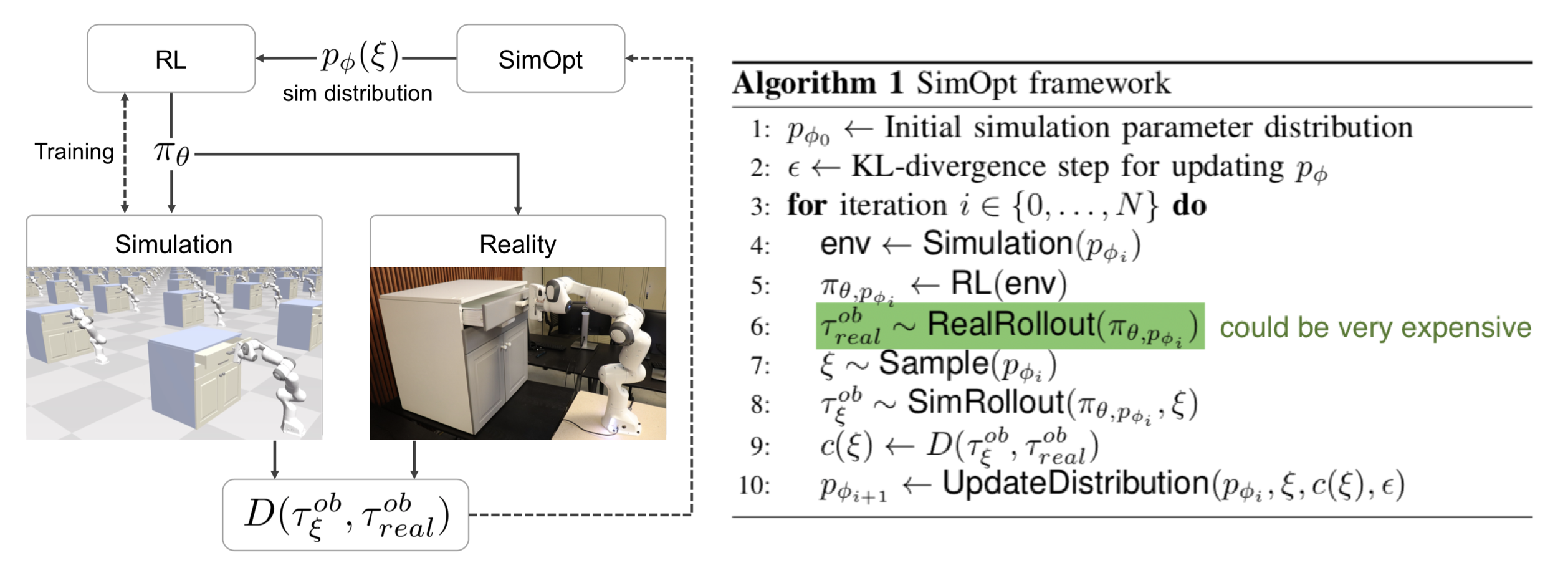
The SimOpt method (Chebotar et al, 2019) is first trained under an initial randomization distribution $P_\phi(\xi)$, producing a policy $\pi_{\theta, P_\phi}$. That policy is then deployed in both the simulator and on a physical robot to collect trajectories $\tau_\xi$ and $\tau_\text{real}$, respectively. The objective is to minimize the discrepancy between simulated and real trajectories:

$ \phi^* = \arg\min_{\phi}\mathbb{E}_{\xi \sim P_\phi(\xi)} [\mathbb{E}_{\pi_{\theta, P_\phi}} [D(\tau_\text{sim}, \tau_\text{real})]] $

where $D(.)$ is a trajectory-based discrepancy metric. As in “Learning to simulate,” SimOpt must address the challenge of propagating gradients through a non-differentiable simulator. It uses a method called relative entropy policy search, see the paper for details.

An overview of the SimOpt framework. (Image source: Chebotar et al, 2019)

RCAN (James et al., 2019), short for “Randomized-to-Canonical Adaptation Networks,” combines DA and DR for end-to-end RL tasks. An image-conditional GAN (cGAN) is trained in simulation to translate a domain-randomized image into a non-randomized version (the “canonical version”). The same model is then used to translate real images into the corresponding simulated version, ensuring that the agent receives observations consistent with what it encountered during training. This approach still relies on the assumption that the distribution of domain-randomized simulated images is broad enough to cover real-world samples.

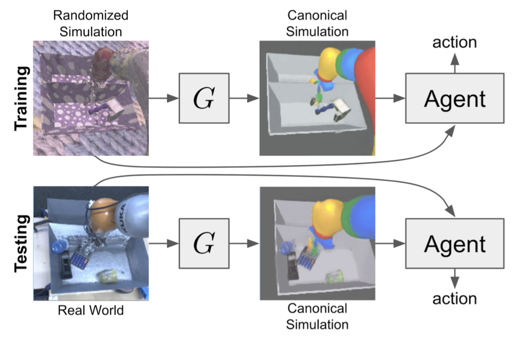
RCAN is an image-conditional generator that can convert a domain-randomized or real image into its corresponding non-randomized simulator version. (Image source: James et al., 2019)

The RL model is trained end-to-end in a simulator for vision-based robot arm grasping. Randomization is applied at every timestep, including tray divider position, the objects to grasp, random textures, and the position, direction, and color of the lighting. The canonical version corresponds to the simulator’s default appearance. RCAN aims to learn a generator

$G$: randomized image $\to$ {canonical image, segmentation, depth}

where segmentation masks and depth images serve as auxiliary tasks. RCAN achieved better zero-shot transfer than uniform DR, although both approaches performed worse than a model trained solely on real images. Conceptually, RCAN operates in the reverse direction of GraspGAN, which uses domain adaptation to translate synthetic images into real ones.

Guided by Data in Simulator

Network-driven domain randomization (Zakharov et al., 2019), also known as DeceptionNet, is motivated by learning which randomizations are actually useful for bridging the domain gap in image classification tasks.

Randomization is implemented through a set of deception modules with an encoder-decoder architecture. These deception modules are designed specifically for image transformations, such as changing backgrounds, adding distortion, or modifying lighting. A separate recognition network performs the main task by classifying the transformed images.

Training proceeds in two steps:

With the recognition network fixed, maximize the difference between predictions and labels by applying reversed gradients during backpropagation, allowing the deception module to learn the most confusing transformations.
With the deception modules fixed, train the recognition network using the altered input images.

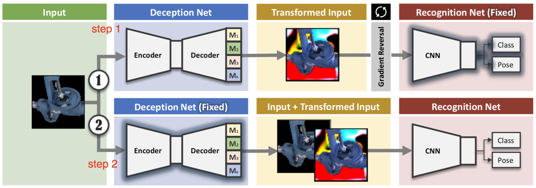
How DeceptionNet works. (Image source: Zakharov et al., 2019)

The downstream classifier supplies the training signal for the deception modules. However, unlike the approach in the section above, these randomization modules are designed to create more difficult cases rather than directly maximizing task performance. A major drawback is that different deception modules must be manually designed for different datasets or tasks, which limits scalability. Despite being zero-shot, the results are still worse than SOTA DA methods on MNIST and LineMOD.

Similarly, Active domain randomization (ADR; Mehta et al., 2019) also uses simulated data to generate more challenging training samples. ADR searches for the most informative environment variations within specified randomization ranges, where informativeness is defined by discrepancies between policy rollouts in randomized environments and rollouts in reference (original, non-randomized) instances. This resembles SimOpt, with an important distinction: SimOpt measures discrepancy between simulation and real rollouts, whereas ADR measures discrepancy between randomized and non-randomized simulation rollouts, thereby avoiding expensive real-world data collection.

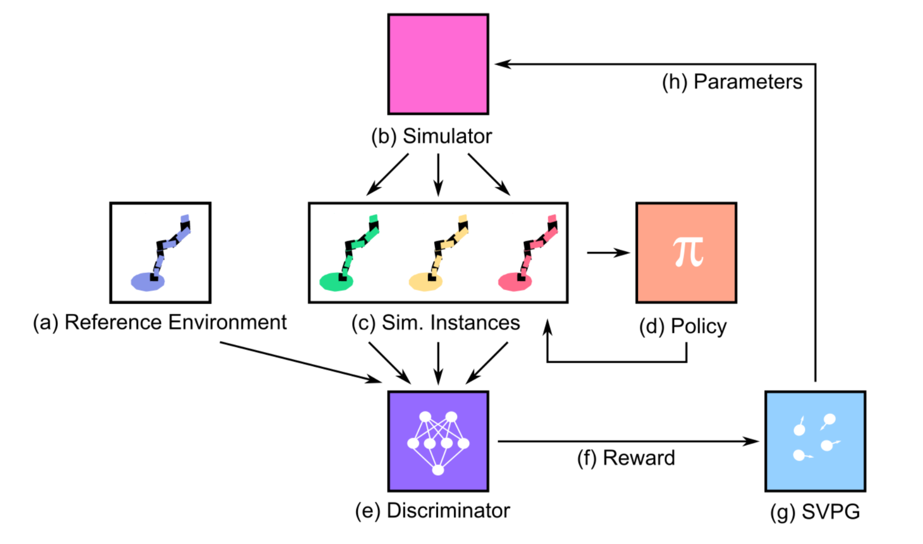
How active domain randomization (ADR) works. (Image source: Mehta et al., 2019)

More precisely, training proceeds as follows:

Given a policy, run it in both reference and randomized environments, collecting two corresponding sets of trajectories.
Train a discriminator to determine whether a rollout trajectory comes from a randomized run or a reference run. The predicted $\log p$ (probability of being randomized) is used as the reward. The more different the randomized and reference rollouts are, the easier the prediction, and the higher the reward.
- The intuition is that if an environment is easy, the same policy produces trajectories similar to those in the reference instance. The method therefore rewards and explores difficult environments by encouraging different behaviors.
Use the discriminator reward as input to Stein Variational Policy Gradient (SVPG) particles, which output a diverse set of randomization configurations.

ADR is an attractive idea, with two minor concerns. When executing a stochastic policy, trajectory similarity may not be an ideal measure of environment difficulty. In addition, the sim2real results are, unfortunately, not as compelling, although the paper argues that ADR’s advantage is its exploration of a smaller range of randomization parameters.

Cited as:

@article{weng2019DR,
  title   = "Domain Randomization for Sim2Real Transfer",
  author  = "Weng, Lilian",
  journal = "lilianweng.github.io",
  year    = "2019",
  url     = "https://lilianweng.github.io/posts/2019-05-05-domain-randomization/"
}

Overall, after reading this post, I hope you like domain randomization as much as I do :).

References

[1] Josh Tobin, et al. “Domain randomization for transferring deep neural networks from simulation to the real world.” IROS, 2017.
[2] Fereshteh Sadeghi and Sergey Levine. “CAD2RL: Real single-image flight without a single real image.” arXiv:1611.04201 (2016).
[3] Xue Bin Peng, et al. “Sim-to-real transfer of robotic control with dynamics randomization.” ICRA, 2018.
[4] Nataniel Ruiz, et al. “Learning to Simulate.” ICLR 2019
[5] OpenAI. “Learning Dexterous In-Hand Manipulation.” arXiv:1808.00177 (2018).
[6] OpenAI Blog. “Learning dexterity” July 30, 2018.
[7] Quan Vuong, et al. “How to pick the domain randomization parameters for sim-to-real transfer of reinforcement learning policies?.” arXiv:1903.11774 (2019).
[8] Ekin D. Cubuk, et al. “AutoAugment: Learning augmentation policies from data.” arXiv:1805.09501 (2018).
[9] Wenhao Yu et al. “Policy Transfer with Strategy Optimization.” ICLR 2019
[10] Yevgen Chebotar et al. “Closing the Sim-to-Real Loop: Adapting Simulation Randomization with Real World Experience.” Arxiv: 1810.05687 (2019).
[11] Stephen James et al. “Sim-to-real via sim-to-sim: Data-efficient robotic grasping via randomized-to-canonical adaptation networks” CVPR 2019.
[12] Bhairav Mehta et al. “Active Domain Randomization” arXiv:1904.04762
[13] Sergey Zakharov,et al. “DeceptionNet: Network-Driven Domain Randomization.” arXiv:1904.02750 (2019).
[14] Amlan Kar, et al. “Meta-Sim: Learning to Generate Synthetic Datasets.” arXiv:1904.11621 (2019).
[15] Aayush Prakash, et al. “Structured Domain Randomization: Bridging the Reality Gap by Context-Aware Synthetic Data.” arXiv:1810.10093 (2018).