[Updated on 2020-01-09: add a new section on Contrastive Predictive Coding].
[Updated on 2020-04-13: add a “Momentum Contrast” section on MoCo, SimCLR and CURL.]
[Updated on 2020-07-08: add a “Bisimulation” section on DeepMDP and DBC.]
[Updated on 2020-09-12: add MoCo V2 and BYOL in the “Momentum Contrast” section.]
[Updated on 2021-05-31: remove section on “Momentum Contrast” and add a pointer to a full post on “Contrastive Representation Learning”]

With a well-defined task and enough labels, supervised learning can perform extremely well. In practice, strong results typically require a substantial volume of labeled examples, but collecting high-quality manual annotations is costly (for example, ImageNet) and difficult to scale. At the same time, unlabeled data (such as free text and the vast number of images on the Internet) is far more abundant than the limited set of human-curated labeled datasets, so ignoring it is inefficient. However, unsupervised learning is challenging and, in many cases, much less sample-efficient than supervised training.

What if we could obtain labels “for free” from unlabeled data, then train on that unlabeled dataset using standard supervised objectives? This is possible by designing a supervised learning problem in a special form: predict only a subset of the information given the rest. In that setup, everything required, both inputs and labels, is already present in the data itself. This approach is known as self-supervised learning.

This idea is widely used in language modeling. A conventional language-model objective is next-token prediction given the preceding sequence. BERT adds two auxiliary tasks, both of which depend on labels generated from the data.

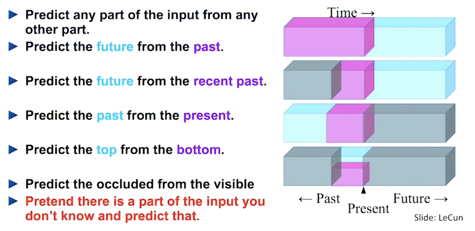
Here is a well-curated list of papers on self-supervised learning. If you would like to explore the literature in more depth, it is a good place to start.

Note that this post does not focus on NLP and language modeling, nor on generative modeling.

Why Self-Supervised Learning?

Self-supervised learning enables us to take advantage of labels that effectively come bundled with the data at no additional cost. The motivation is straightforward: building a dataset with clean, reliable labels is expensive, whereas unlabeled data is produced continuously. To capitalize on this much larger pool of unlabeled data, one approach is to define learning objectives that extract supervision directly from the data itself.

A self-supervised task, also called a pretext task, provides a supervised loss signal. In most cases, the final accuracy on the invented task is not the goal. Instead, the primary interest is the intermediate representation learned by the model. The hope is that this representation captures useful semantics or structure and transfers well to a range of real downstream tasks.

For example, we can randomly rotate images and train a model to predict the rotation applied to each input. Because rotation prediction is an artificial task, its raw accuracy is not the main objective (similar to typical auxiliary tasks). The expectation is that the model will learn high-quality latent variables that support real applications, such as object recognition with very few labeled examples.

Broadly, many generative models can be viewed as self-supervised, but with different end goals: generative models emphasize producing diverse, realistic samples, whereas self-supervised representation learning emphasizes learning generally useful features. Generative modeling is not the focus of this post; however, you can refer to my previous posts.

Images-Based

A wide range of ideas have been proposed for self-supervised representation learning on images. A common evaluation workflow is to train a model on one or more pretext tasks using unlabeled images, then take an intermediate feature layer as input to a multinomial logistic regression classifier for ImageNet classification. The resulting classification accuracy serves as a proxy for the quality of the learned representation.

More recently, some work has proposed training supervised objectives on labeled data and self-supervised pretext tasks on unlabeled data simultaneously using shared weights, as in Zhai et al, 2019 and Sun et al, 2019.

Distortion

The underlying assumption is that small distortions applied to an image should not change its semantic meaning or overall geometric structure. Therefore, lightly distorted versions of an image can be treated as equivalent to the original, and the learned features are expected to be invariant to these distortions.

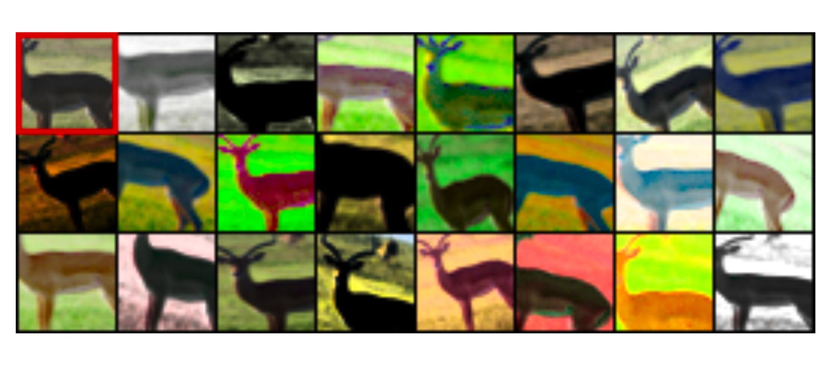
Exemplar-CNN (Dosovitskiy et al., 2015) builds a surrogate training dataset from unlabeled image patches:

1. Sample $N$ patches of size 32 × 32 pixels from different images at varying positions and scales, selecting only regions with substantial gradients, since these areas contain edges and tend to include objects or object parts. These are referred to as “exemplary” patches.
2. Apply a variety of random transformations to each patch (for example, translation, rotation, scaling, etc.). All distorted variants are treated as belonging to the same surrogate class.
3. The pretext task is to discriminate among surrogate classes. The number of surrogate classes can be chosen arbitrarily.

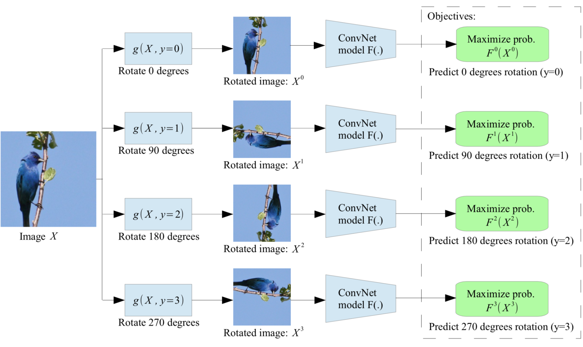
Rotation of an entire image (Gidaris et al. 2018) is another inexpensive and effective way to alter an input while keeping the semantic content intact. Each input image is randomly rotated by a multiple of $90^\circ$, corresponding to $[0^\circ, 90^\circ, 180^\circ, 270^\circ]$. The model is trained to predict which rotation was applied, yielding a 4-class classification problem.

To recognize the same image across different rotations, the model must learn higher-level object components (for example, heads, noses, and eyes) and their relative arrangement, rather than relying only on local texture patterns. In this way, the pretext task encourages the model to learn semantic object concepts.

Patches

A second category of self-supervised tasks extracts multiple patches from a single image and trains the model to predict relationships among those patches.

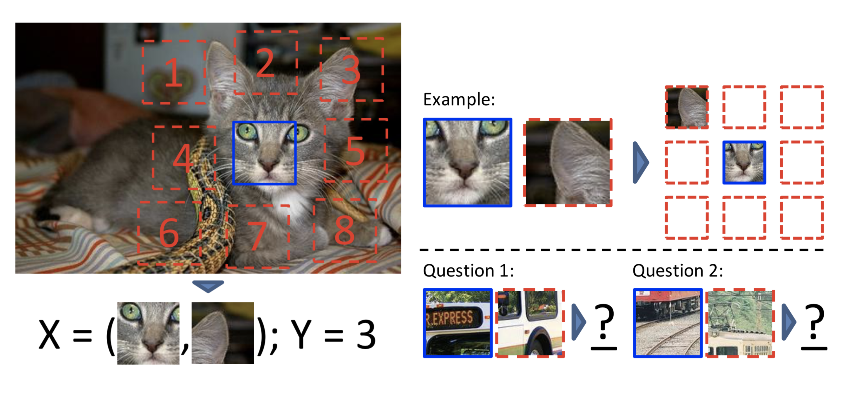
Doersch et al. (2015) formulates a pretext task that predicts the relative position between two random patches sampled from the same image. To succeed, a model must capture the spatial context of objects to infer how parts relate spatially.

Patches are sampled as follows:

1. Randomly sample the first patch without conditioning on image content.
2. Assume the first patch lies at the center of a 3x3 grid, then sample the second patch from one of the eight neighboring grid locations.
3. To prevent the model from exploiting low-level shortcuts (for example, connecting a straight line across patch boundaries or matching local textures), introduce additional noise by:
   • Adding gaps between patches
   • Applying small jitters
   • Randomly downsampling some patches to as few as 100 total pixels, then upsampling them, to improve robustness to pixelation
   • Shifting green and magenta toward gray or randomly dropping 2 of 3 color channels (see “chromatic aberration” below)
4. Train the model to predict which of the eight neighboring locations the second patch comes from, an 8-class classification problem.

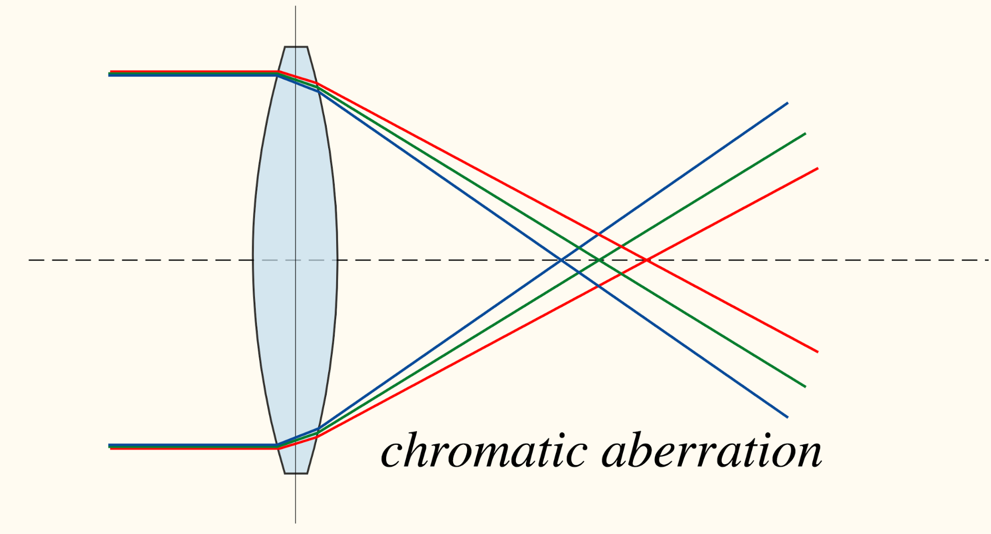
Beyond trivial cues such as boundary continuation or repeating textures, another surprisingly effective shortcut was identified: “chromatic aberration”. This effect arises because light of different wavelengths can have different focal lengths through a lens, producing small offsets among color channels. As a result, a model may infer relative position merely by comparing how green and magenta are misaligned between two patches. This solution is unrelated to image content and is therefore undesirable. Preprocessing images by shifting green and magenta toward gray, or randomly dropping 2 of 3 color channels, can mitigate this shortcut.

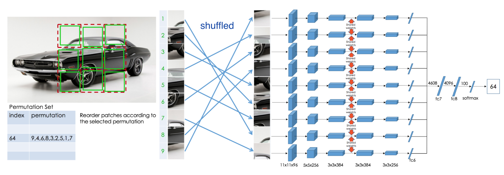
Given the 3x3 grid setup in the task above, one natural extension is to use all nine patches rather than only two, thereby increasing task difficulty. Building on this idea, Noroozi & Favaro (2016) proposed a jigsaw puzzle pretext task: train the model to restore nine shuffled patches to their original positions.

A convolutional network processes each patch independently using shared weights, then outputs a probability vector corresponding to the patch index within a predefined permutation set. To control puzzle difficulty, the paper shuffles patches using a predefined set of permutations and configures the model to predict a probability distribution over permutation indices in that set.

Because the patch shuffling does not change the correct target ordering to predict, a potential speedup is to use a permutation-invariant graph convolutional network (GCN), so the same set of patches does not need to be reshuffled repeatedly, following the same idea as in this paper.

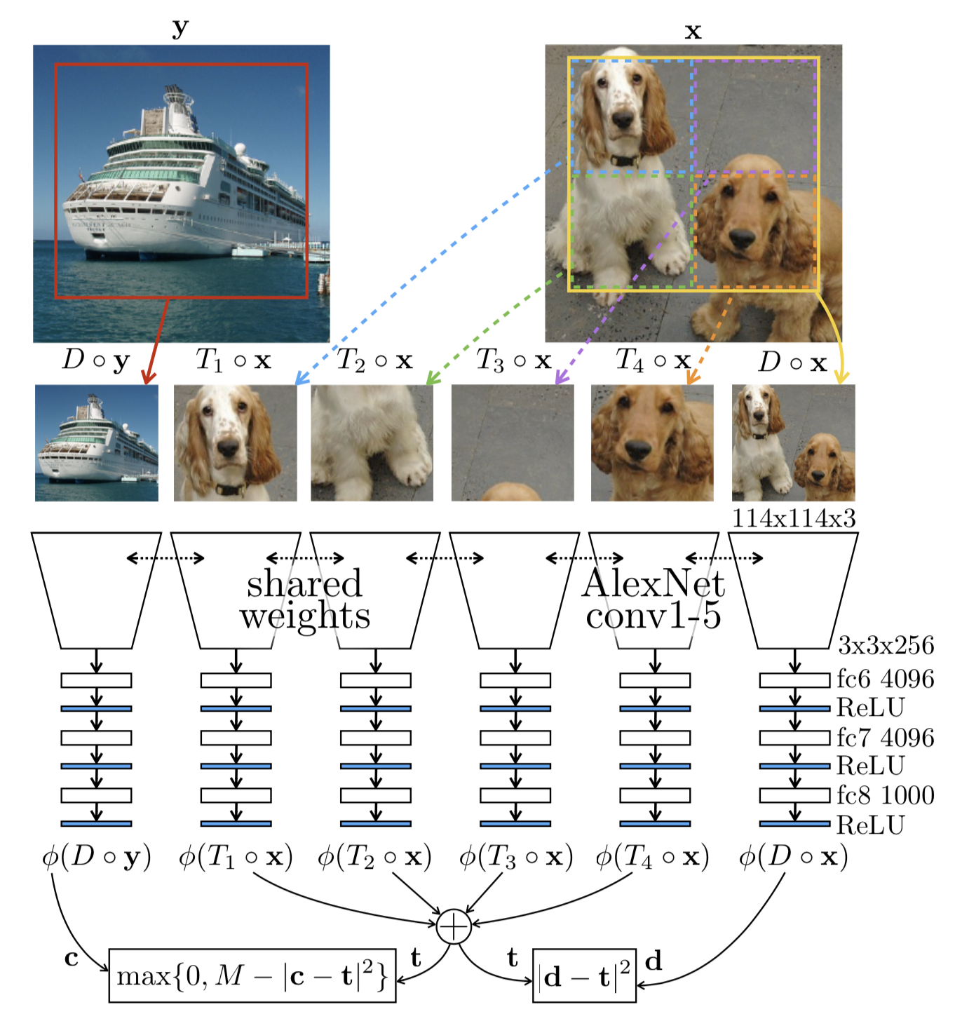
Another approach treats a “feature” or “visual primitive” as a scalar attribute that can be summed over patches and compared across them. Under this view, relationships among patches can be defined through counting features and basic arithmetic (Noroozi, et al, 2017).

The paper uses two transformations:

1. Scaling: If an image is scaled up by 2x, the number of visual primitives should remain unchanged.
2. Tiling: If an image is tiled into a 2x2 grid, the number of visual primitives should add up accordingly, yielding four times the original feature count.

The model learns a feature encoder $\phi(.)$ from this feature-counting relationship. Given an input image $\mathbf{x} \in \mathbb{R}^{m \times n \times 3}$, consider two types of transformation operators:

1. Downsampling operator, $D: \mathbb{R}^{m \times n \times 3} \mapsto \mathbb{R}^{\frac{m}{2} \times \frac{n}{2} \times 3}$: downsample by a factor of 2
2. Tiling operator $T_i: \mathbb{R}^{m \times n \times 3} \mapsto \mathbb{R}^{\frac{m}{2} \times \frac{n}{2} \times 3}$: extract the $i$-th tile from a 2x2 grid of the image.

We expect to learn:

Thus the MSE loss is: $\mathcal{L}_\text{feat} = |\phi(D \circ \mathbf{x}) - \sum_{i=1}^4 \phi(T_i \circ \mathbf{x})|^2_2$. To avoid trivial solution $\phi(\mathbf{x}) = \mathbf{0}, \forall{\mathbf{x}}$, another loss term is added to encourage the difference between features of two different images: $\mathcal{L}_\text{diff} = \max(0, c -|\phi(D \circ \mathbf{y}) - \sum_{i=1}^4 \phi(T_i \circ \mathbf{x})|^2_2)$, where $\mathbf{y}$ is another input image different from $\mathbf{x}$ and $c$ is a scalar constant. The final loss is:

Noroozi, et al, 2017)

Colorization

Colorization can serve as a strong self-supervised task. Here, a model is trained to colorize a grayscale input image. More precisely, the objective is to map the grayscale input to a probability distribution over quantized color values (Zhang et al. 2016).

The model predicts colors in the CIE Lab* color space. Lab* is designed to approximate human vision, whereas RGB or CMYK primarily model the color output characteristics of physical devices.

• The L* component corresponds to perceived lightness, L* = 0 is black, and L* = 100 indicates white.
• The a* component represents green (negative) versus magenta (positive).
• The b* component represents blue (negative) versus yellow (positive).

Because colorization is inherently multimodal, optimizing cross-entropy over a predicted distribution of binned color values performs better than an L2 loss on raw color values. The ab color space is quantized with bucket size 10.

To balance frequent colors (typically low ab values associated with common backgrounds such as clouds, walls, and dirt) against rare colors (often tied to key objects), the loss is reweighted to upweight infrequent color buckets. This parallels the motivation for using both tf and idf when scoring words in information retrieval. The weighting term is defined as: (1-λ) * Gaussian-kernel-smoothed empirical probability distribution + λ * a uniform distribution, where both distributions are over the quantized ab color space.

Generative Modeling

In generative modeling, the pretext task is to reconstruct the original input, while learning a latent representation that captures meaningful structure.

A denoising autoencoder (Vincent, et al, 2008) is trained to recover an image from a partially corrupted or noise-injected version. The design is motivated by the observation that humans can recognize objects even in noisy images, suggesting that key visual features can be extracted and separated from noise. See my old post.

A context encoder (Pathak, et al., 2016) is trained to fill in missing regions of an image. Let $\hat{M}$ be a binary mask, where 0 denotes dropped pixels and 1 denotes remaining input pixels. Training uses a combination of reconstruction (L2) loss and adversarial loss. The removed regions specified by the mask can take arbitrary shapes.

where $F(.)$ is the full impainting pipeline for reconstructing the image with missing regions, including both encoder and decoder portions in $D(.)$ is the discriminator model trained jointly, as in GAN.

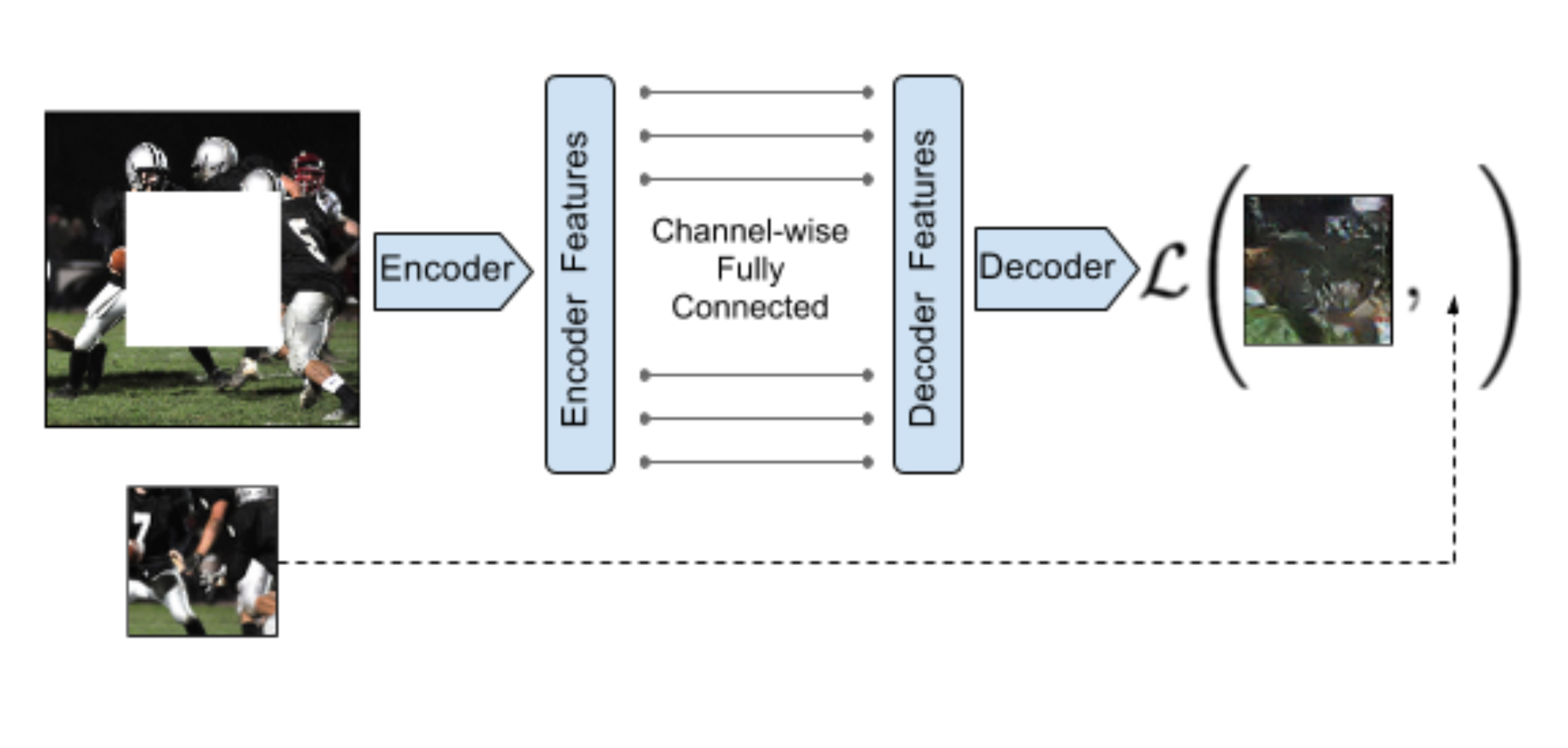
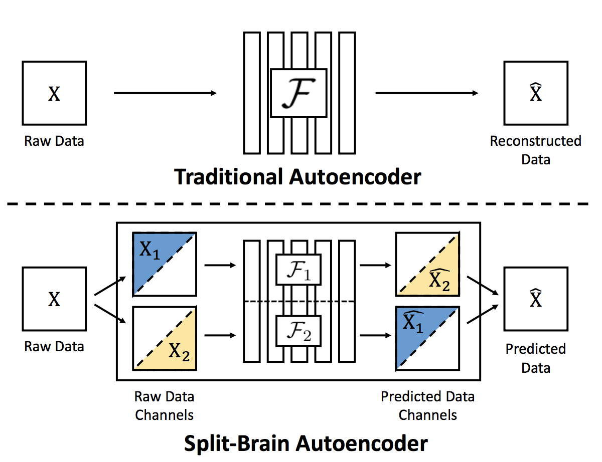
When masking an image, the context encoder removes all color-channel information in selected regions. What if we instead hide only a subset of channels? The split-brain autoencoder (Zhang et al., 2017) follows this approach by predicting a subset of color channels from the remaining channels. Let the data tensor $\mathbf{x} \in \mathbb{R}^{h \times w \times \vert C \vert }$ with $C$ color channels be the input to the $l$-th layer of the network. Split it into two disjoint parts, $\mathbf{x}_1 \in \mathbb{R}^{h \times w \times \vert C_1 \vert}$ and $\mathbf{x}_2 \in \mathbb{R}^{h \times w \times \vert C_2 \vert}$, where $C_1 , C_2 \subseteq C$. Then train two subnetworks to perform complementary predictions: one network $f_1$ predicts $\mathbf{x}_2$ from $\mathbf{x}_1$, and the other network $f_1$ predicts $\mathbf{x}_1$ from $\mathbf{x}_2$. The loss is either an L1 loss, or cross-entropy if color values are quantized.

The split may be performed once in RGB-D or Lab* color space, or it can occur at every layer of a CNN, where the channel count may be arbitrary.

Generative adversarial networks (GANs) can learn mappings from simple latent variables to arbitrarily complex data distributions. Prior studies suggest that the latent space learned by such generative models captures semantic variation in the data. For example, when GANs are trained on human faces, certain latent variables correlate with attributes such as facial expression, glasses, and gender (Radford et al., 2016).

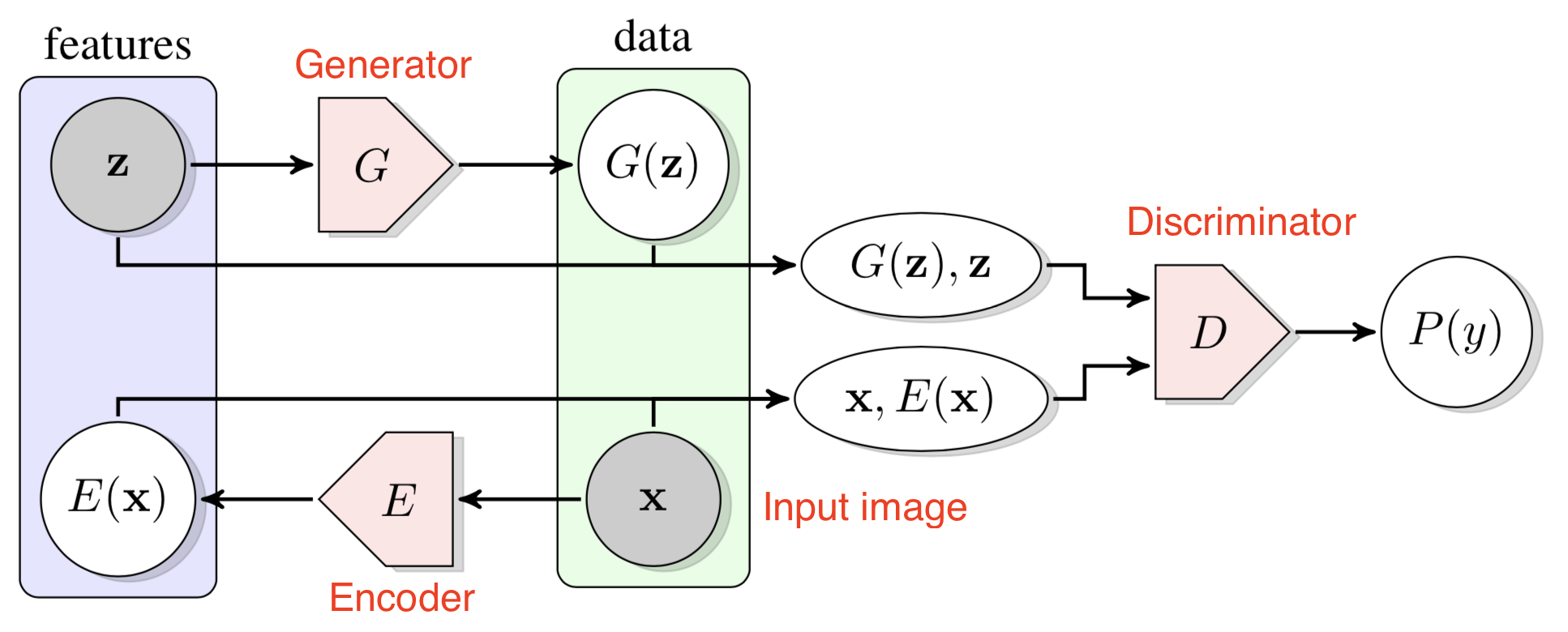
Bidirectional GANs (Donahue, et al, 2017) add an encoder $E(.)$ to learn the mapping from an input to a latent variable $\mathbf{z}$. The discriminator $D(.)$ operates in the joint space of input data and latent representation, $(\mathbf{x}, \mathbf{z})$, and distinguishes the generated pair $(\mathbf{x}, E(\mathbf{x}))$ from the real pair $(G(\mathbf{z}), \mathbf{z})$. Training optimizes the objective $\min_{G, E} \max_D V(D, E, G)$, where the generator $G$ and the encoder $E$ learn to produce data and latent variables realistic enough to confuse the discriminator, while the discriminator $D$ learns to distinguish real from generated examples.

Contrastive Learning

Contrastive Predictive Coding (CPC) (van den Oord, et al. 2018) is an approach to unsupervised learning from high-dimensional data that reframes a generative modeling objective as a classification problem. CPC uses a contrastive loss, also called the InfoNCE loss. Inspired by Noise Contrastive Estimation (NCE), this loss applies cross-entropy to measure how effectively the model can identify a “future” representation among a set of unrelated “negative” samples. This design is partly motivated by the observation that unimodal losses such as MSE may be insufficiently expressive, while learning a full generative model can be prohibitively expensive.

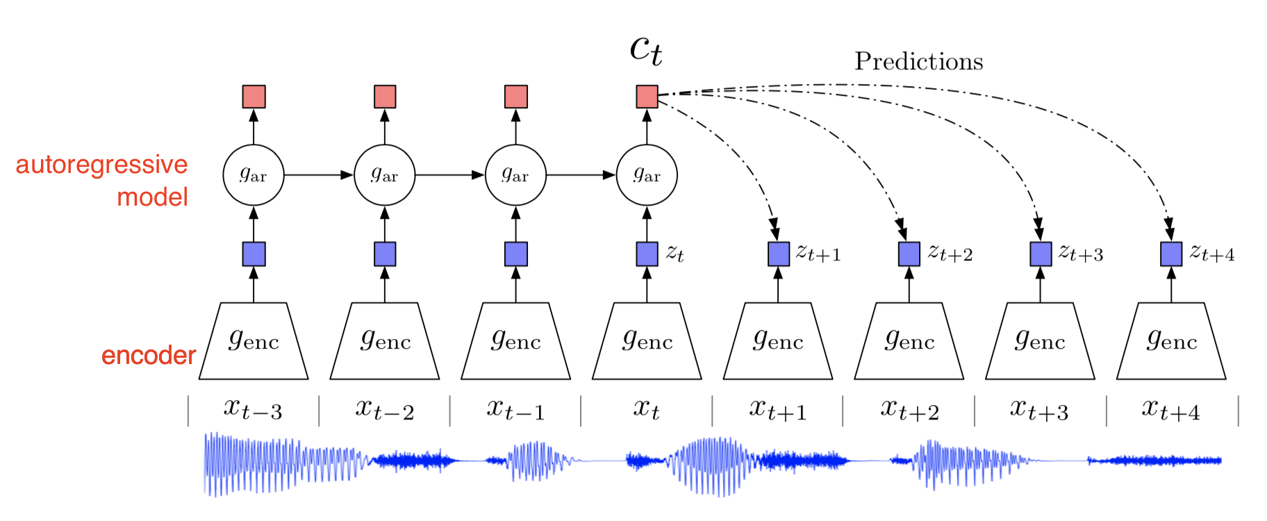
CPC uses an encoder to compress input data $z_t = g_\text{enc}(x_t)$ and an autoregressive decoder to learn a higher-level context representation that may be shared across future predictions, $c_t = g_\text{ar}(z_{\leq t})$. End-to-end training relies on an NCE-inspired contrastive loss.

When predicting future information, CPC is optimized to maximize the mutual information between the input $x$ and the context vector $c$:

Instead of explicitly modeling future observations $p_k(x_{t+k} \vert c_t)$ (which may be expensive), CPC models a density function that preserves mutual information between $x_{t+k}$ and $c_t$:

where $f_k$ may be unnormalized, and a linear transformation $W_k^\top c_t$ is used for prediction with a different $W_k$ matrix for each step $k$.

Given a set of $N$ random samples $X = \{x_1, \dots, x_N\}$ that contains one positive sample $x_t \sim p(x_{t+k} \vert c_t)$ and $N-1$ negative samples $x_{i \neq t} \sim p(x_{t+k})$, the cross-entropy loss for correctly classifying the positive sample (where $\frac{f_k}{\sum f_k}$ is the prediction) is:

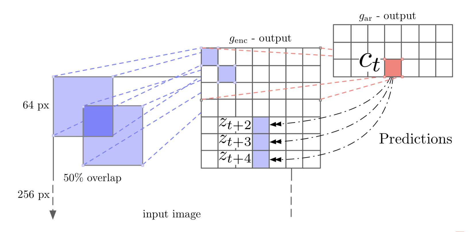
When applying CPC to images (Henaff, et al. 2019), the predictor network must operate on a masked feature set to prevent trivial predictions. Concretely:

1. Divide each input image into a set of overlapping patches, and encode each patch using a ResNet encoder to obtain compressed feature vectors $z_{i,j}$.
2. Use a masked convolutional network to ensure that the receptive field of each output neuron can only access content above it in the image. Without this constraint, prediction would become trivial. Predictions can be made in both directions (top-down and bottom-up).
3. Predict $z_{i+k, j}$ from context $c_{i,j}$: $\hat{z}_{i+k, j} = W_k c_{i,j}$.

A contrastive loss evaluates the prediction by encouraging the model to correctly identify the target among negative representations $\{z_l\}$ sampled from other patches in the same image and from other images in the same batch:

For additional discussion of contrastive learning, see the post on “Contrastive Representation Learning”.

Video-Based

A video is a sequence of semantically related frames. Frames that are close in time tend to be more strongly correlated than frames that are farther apart. Frame order also encodes regularities in reasoning and physical logic, for example, object motion should be smooth and gravity points downward.

A widely used workflow is to pretrain a model on one or more pretext tasks using unlabeled video, then extract features from an intermediate layer and use them to fine-tune a lightweight model for downstream tasks such as action classification, segmentation, or object tracking.

Tracking

Object motion can be followed across a sequence of frames. Between adjacent frames, the visual change for the same object is typically small, often due to minor object motion or camera motion. As a result, any learned representation for the same object across nearby frames should remain close in latent feature space. Based on this intuition, Wang & Gupta, 2015 proposed an approach for unsupervised visual representation learning by tracking moving objects in video.

Concretely, patches exhibiting motion are tracked over a short temporal window (for example, 30 frames). The first patch $\mathbf{x}$ and the last patch $\mathbf{x}^+$ are selected and treated as a training pair. If the model is trained only to minimize the difference between the feature vectors of these two patches, it could collapse to a trivial solution by mapping all inputs to the same value. To prevent this, as in above, a randomly sampled third patch $\mathbf{x}^-$ is introduced. The representation is learned by enforcing that the distance between the two tracked patches is smaller than the distance between the first patch and the random patch in feature space, $D(\mathbf{x}, \mathbf{x}^-)) > D(\mathbf{x}, \mathbf{x}^+)$, where $D(.)$ is the cosine distance:

The loss function is:

Here, $M$ is a scalar constant that sets the minimum required margin between the two distances ($M=0.5$ in the paper). At the optimum, the loss encourages $D(\mathbf{x}, \mathbf{x}^-) >= D(\mathbf{x}, \mathbf{x}^+) + M$.

This loss form is also referred to as triplet loss in face recognition, where the dataset contains images of many people from multiple camera viewpoints. Let $\mathbf{x}^a$ be an anchor image of a given person, $\mathbf{x}^p$ be a positive image of the same person from another angle, and $\mathbf{x}^n$ be a negative image of a different person. In the embedding space, $\mathbf{x}^a$ should be closer to $\mathbf{x}^p$ than to $\mathbf{x}^n$:

A closely related variant of triplet loss, called n-pair loss, is also widely used to learn observation embeddings in robotics. See a later section for additional related material.

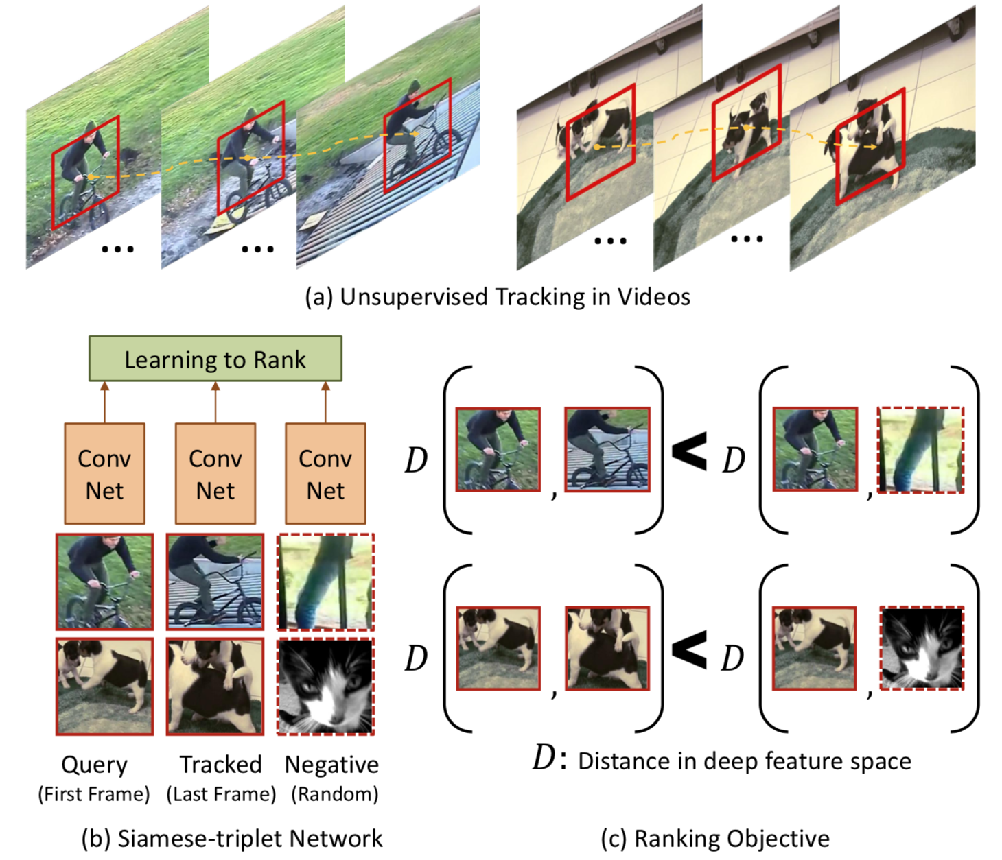
Relevant patches are tracked and extracted using a two-stage, unsupervised optical flow pipeline:

1. Detect SURF interest points and use IDT to estimate the motion of each SURF point.
2. Using the trajectories of the SURF interest points, label points as moving when the flow magnitude exceeds 0.5 pixels.

During training, for a correlated pair of patches $\mathbf{x}$ and $\mathbf{x}^+$, $K$ random patches $\{\mathbf{x}^-\}$ are sampled within the same batch, yielding $K$ training triplets. After a few epochs, hard negative mining is used to make training more challenging and efficient: the method searches for random patches that maximize the loss and uses them for gradient updates.

Frame Sequence

Video frames are naturally ordered in time. Several self-supervised objectives leverage the assumption that a strong representation should encode the correct sequence of frames.

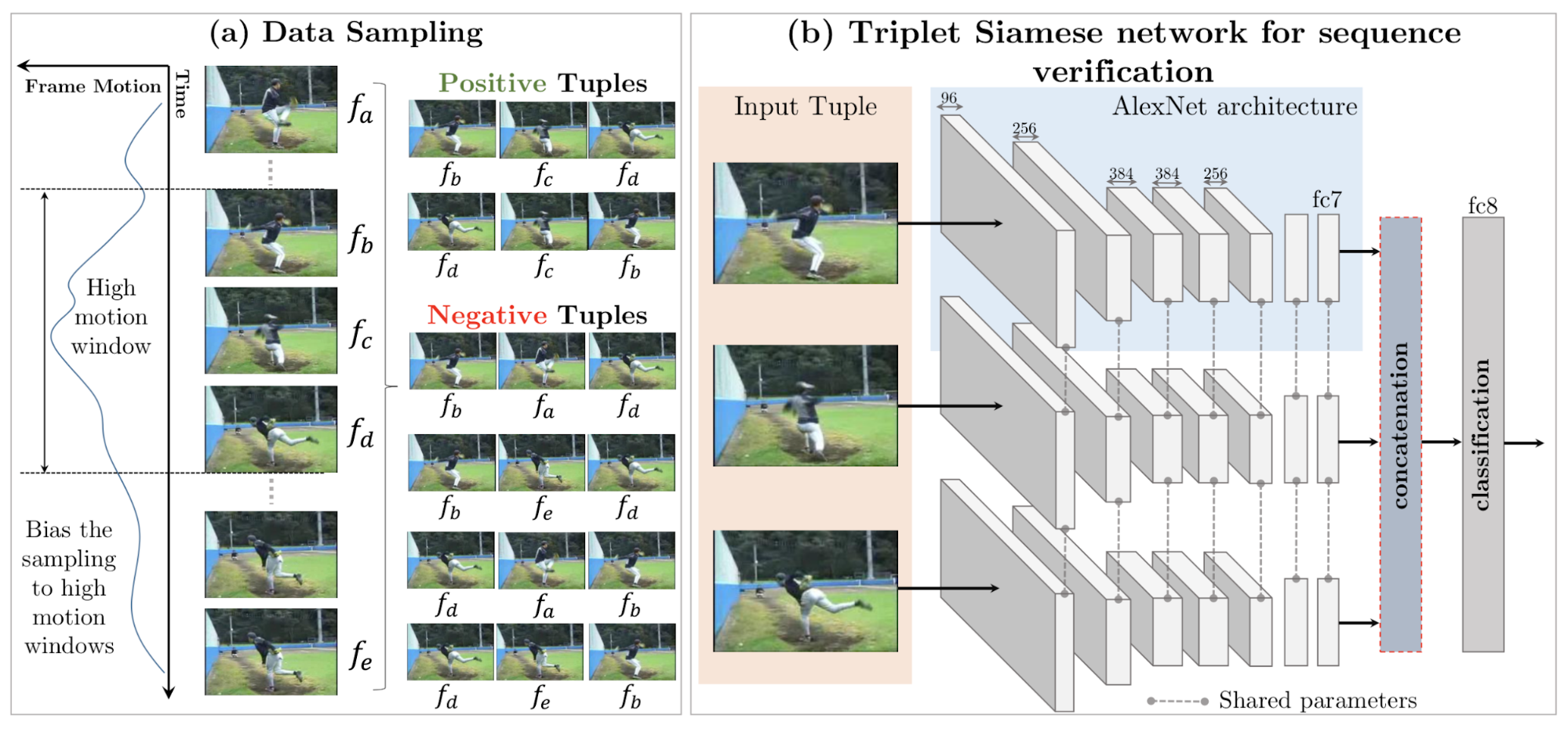
One approach is to validate frame order (Misra, et al 2016). The pretext task is to decide whether a sampled sequence of frames from a video is in correct temporal order (“temporal valid”). Solving this task requires the model to track and reason about subtle object motion across frames.

Training frames are drawn from high-motion windows. Each time, 5 frames are sampled $(f_a, f_b, f_c, f_d, f_e)$, with timestamps that satisfy $a < b < c < d < e$. From these 5 frames, the construction yields one positive tuple $(f_b, f_c, f_d)$ and two negative tuples, $(f_b, f_a, f_d)$ and $(f_b, f_e, f_d)$. The parameter $\tau_\max = \vert b-d \vert$ controls the difficulty of positive examples (that is, higher → harder), and $\tau_\min = \min(\vert a-b \vert, \vert d-e \vert)$ controls the difficulty of negative examples (that is, lower → harder).

This pretext task, validating video frame order, is reported to improve downstream action recognition performance when used for pretraining.

The O3N task (Odd-One-Out Network; Fernando et al. 2017) is also built on frame sequence validation. Extending the prior setup, the objective is to identify the incorrect sequence among multiple video clips.

Given $N+1$ input clips, one clip has its frames shuffled (and is therefore out of order), while the remaining $N$ clips preserve correct temporal order. O3N learns to predict which clip is the odd one out. In the reported experiments, there are 6 input clips, each containing 6 frames.

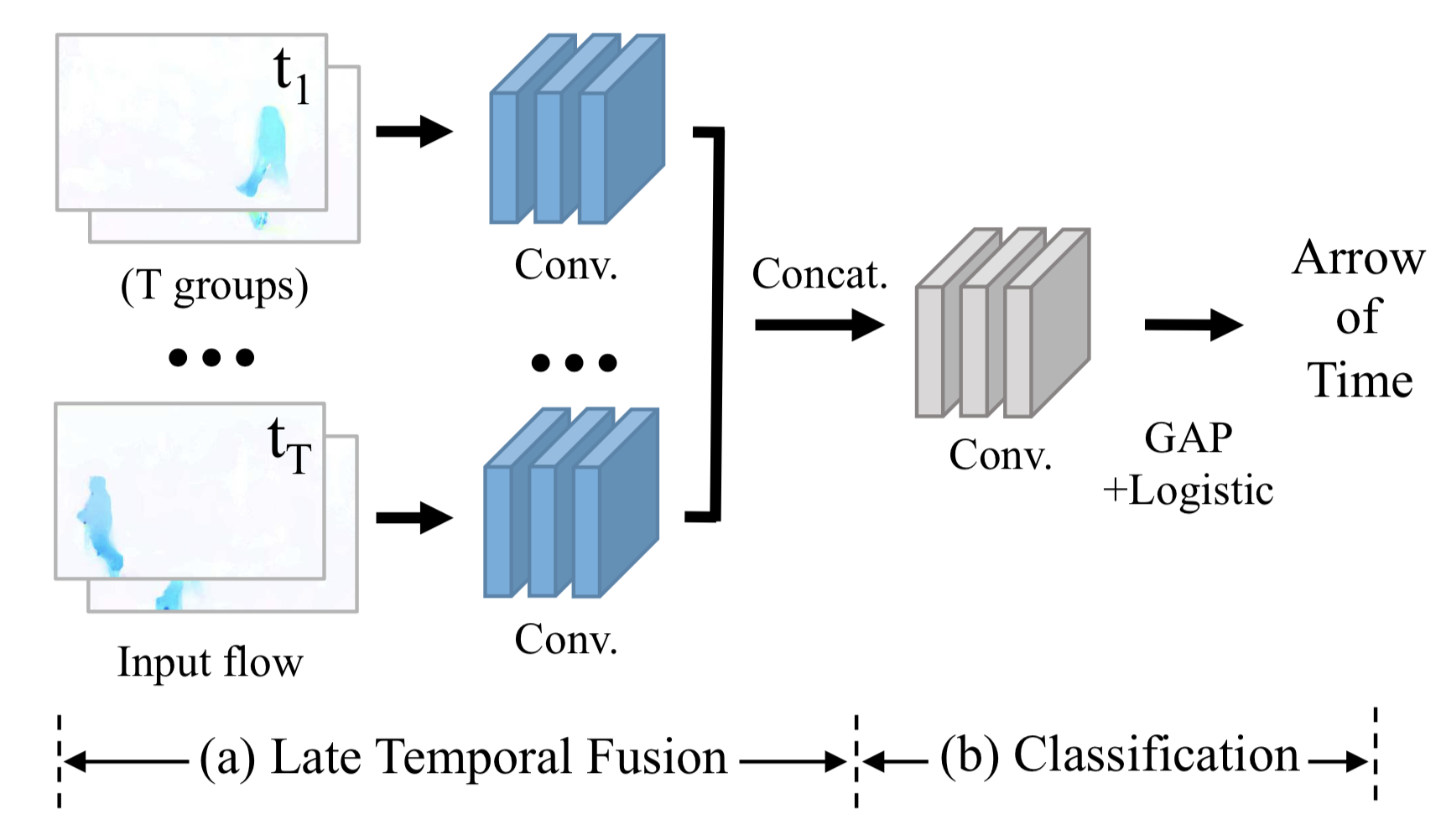
The arrow of time in video also carries informative structure, including low-level physics (for example, gravity pulls objects toward the ground; smoke rises; water flows downward) and high-level event reasoning (for example, fish swim forward; you can break an egg but cannot undo it). This motivates learning representations by predicting the arrow of time (AoT), namely whether the video is played forward or backward (Wei et al., 2018).

To predict the arrow of time, a classifier must capture both low-level physical cues and higher-level semantics. The proposed T-CAM (Temporal Class-Activation-Map) network takes $T$ groups as input, where each group contains multiple optical-flow frames. Convolutional outputs from each group are concatenated and passed to a binary logistic regression head to predict the arrow of time.

Notably, the dataset can include several artificial cues that, if left unaddressed, can enable a trivial classifier that does not depend on true video content:

• Because of video compression artifacts, black framing may not be perfectly black and can leak information about chronological order. Therefore, black framing should be removed in experiments.
• Strong camera motion (such as vertical translation or zooming in and out) can also provide powerful signals for arrow-of-time prediction that are unrelated to scene content. Therefore, the preprocessing pipeline should stabilize camera motion.

The AoT pretext task is shown to improve action classification performance when used for pretraining. Note that fine-tuning is still required.

Video Colorization

Vondrick et al. (2018) proposed video colorization as a self-supervised learning objective. It produces a rich representation that can be used for video segmentation and unlabeled visual region tracking without extra fine-tuning.

In contrast to image-based colorization, this task copies color from a reference frame (in color) to a target frame (in grayscale), exploiting the natural temporal consistency of color across video frames (so the two frames should not be too far apart in time). To copy color reliably across time, the model is structured to learn how to track corresponding pixels between frames.

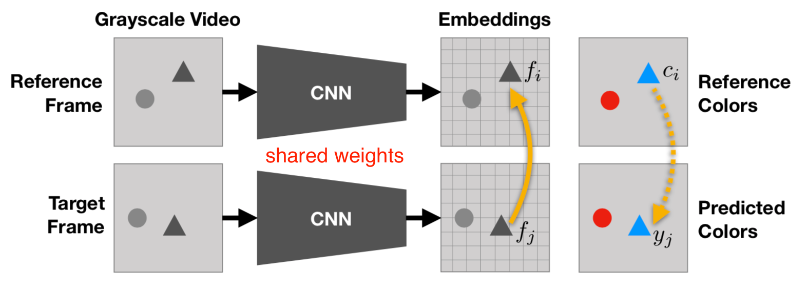
The core mechanism is straightforward and effective. Let $c_i$ denote the true color of the $i-th$ pixel in the reference frame, and let $c_j$ denote the color of the $j$-th pixel in the target frame. The model predicts the color of the $j$-th pixel in the target $\hat{c}_j$ as a weighted sum over the colors of all pixels in the reference frame, where the weights measure similarity:

Here, $f$ are learned embeddings for the corresponding pixels, and $i’$ indexes all pixels in the reference frame. The weighting term acts as an attention-based pointing mechanism, similar to a matching network and a pointer network. Because the full similarity matrix can be very large, both frames are downsampled. Training uses categorical cross-entropy between $c_j$ and $\hat{c}_j$ with quantized colors, as in Zhang et al. 2016.

Depending on how the reference frame is annotated, the model can be applied to several color-driven downstream tasks, including tracking segmentation and tracking human pose over time. No fine-tuning is required. See

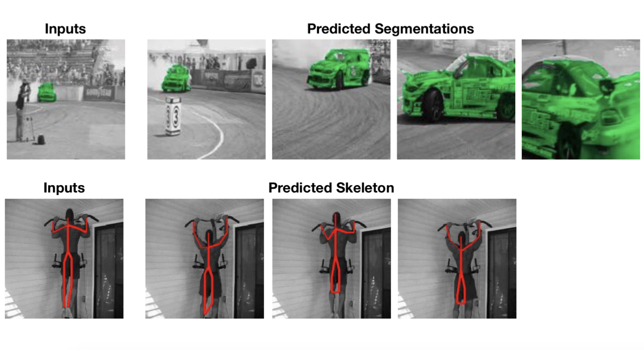
A couple common observations:

• Combining multiple pretext tasks improves performance;
• Deeper networks improve the quality of representation;
• Supervised learning baselines still beat all of them by far.

Control-Based

When executing an RL policy in the real world, such as controlling a physical robot from visual input, it is non-trivial to track state accurately, obtain reliable reward signals, or determine whether a goal has truly been achieved. Visual observations contain substantial noise that is irrelevant to the underlying state, and state equivalence cannot be determined via pixel-level comparison alone. Self-supervised representation learning has demonstrated strong potential for producing useful state embeddings that can be used directly as inputs to a control policy.

All examples discussed in this section come from robotic learning, primarily focusing on state representation from multiple camera views and on goal representation.

Multi-View Metric Learning

Metric learning has appeared repeatedly in the previous sections. The common setup is: given a triplet of samples (anchor $s_a$, positive sample $s_p$, negative sample $s_n$), the learned embedding $\phi(s)$ is trained so that $s_a$ remains close to $s_p$ but far from $s_n$ in latent space.

Grasp2Vec (Jang & Devin et al., 2018) aims to learn an object-centric visual representation for robot grasping from free, unlabeled grasping interactions. Here, object-centric means that, regardless of changes in environment appearance or robot configuration, images containing similar items should be mapped to similar embeddings, while embeddings for dissimilar items should be far apart.

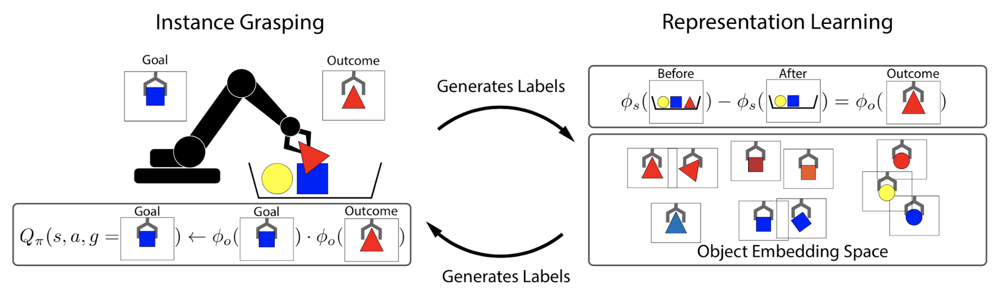
The grasping system can detect whether an object was moved, but it cannot identify which object it moved. Cameras capture images of the full scene and of the grasped object. Early in training, the robot grasps any object $o$ at random, producing an image triplet $(s_\text{pre}, s_\text{post}, o)$:

• $o$: an image of the grasped object held up to the camera
• $s_\text{pre}$: an image of the scene before grasping, with the object $o$ in the tray
• $s_\text{post}$: an image of the same scene after grasping, with the object $o$ removed from the tray

To learn object-centric representations, the approach expects the difference between the embeddings of $s_\text{pre}$ and $s_\text{post}$ to encode the removed object $o$. This idea resembles relationships observed in word embedding, e.g. distance(“king”, “queen”) ≈ distance(“man”, “woman”).

Let $\phi_s$ and $\phi_o$ denote the embedding functions for the scene and the object, respectively. The model learns by minimizing the distance between $\phi_s(s_\text{pre}) - \phi_s(s_\text{post})$ and $\phi_o(o)$ using n-pair loss:

where $B$ denotes a batch of (anchor, positive) pairs.

In metric-learning formulations, n-pair loss is a common choice. Instead of explicitly constructing (anchor, positive, negative) triplets, n-pair loss treats the other positive instances within a mini-batch, across pairs, as negatives.

The embedding function $\phi_o$ is effective for representing a goal $g$ using an image. The reward function measuring how close the actually grasped object $o$ is to the goal is defined as $r = \phi_o(g) \cdot \phi_o(o)$. Reward computation depends only on the learned latent space and does not require ground-truth positions, enabling training on real robots.

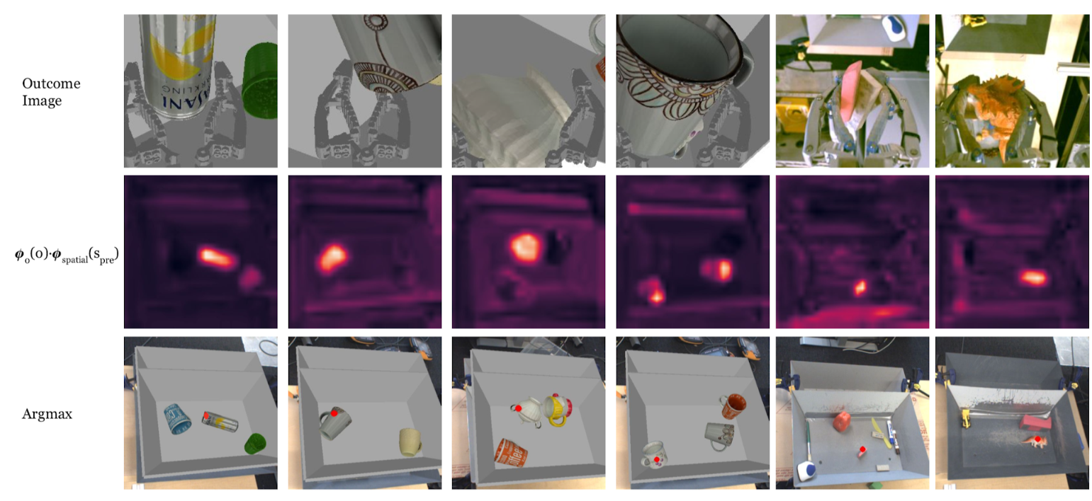
In addition to the embedding-similarity reward, grasp2vec uses several additional techniques when training the RL policy:

• Posthoc labeling: Expand the dataset by treating a randomly grasped object as the correct goal, similar to HER (Hindsight Experience Replay; Andrychowicz, et al., 2017).
• Auxiliary goal augmentation: Further expand the replay buffer by relabeling transitions with goals that were not achieved. Specifically, in each iteration two goals are sampled $(g, g’)$, and both are used to add new transitions to the replay buffer.

TCN (Time-Contrastive Networks; Sermanet, et al. 2018) learn from multi-camera videos using the intuition that different viewpoints of the same scene at the same timestep should share the same embedding (as in FaceNet), while embeddings should change over time, even within the same camera view. In this way, the embedding captures semantic aspects of the underlying state rather than superficial visual similarity. TCN trains the embedding using triplet loss.

Training data is collected by recording the same scene simultaneously from multiple viewpoints. The videos are unlabeled.

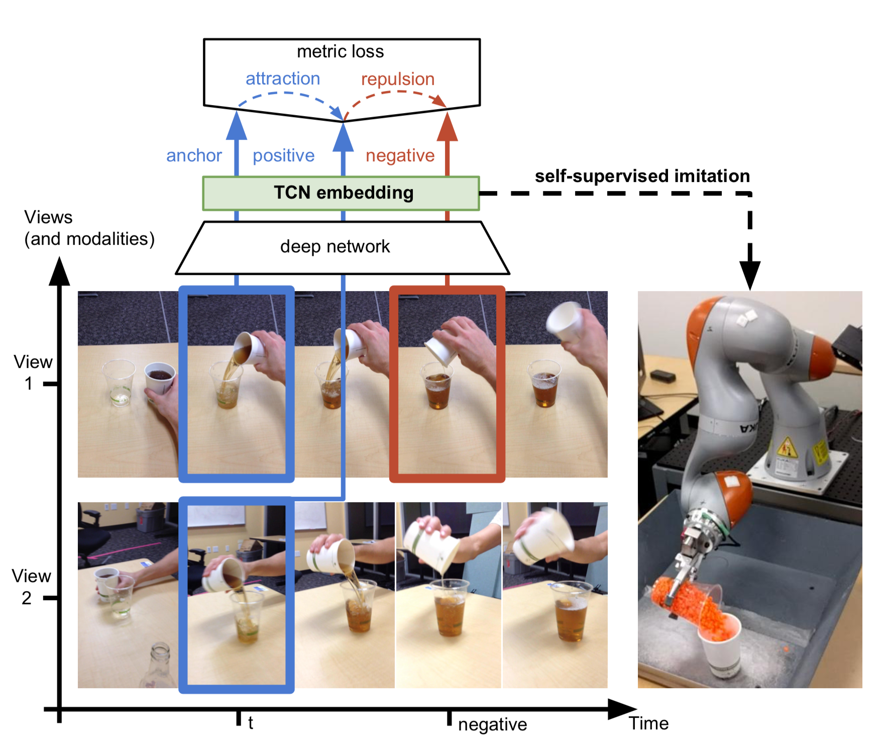
TCN embeddings extract visual features that are invariant to camera configuration. They can be used to define a reward function for imitation learning, based on Euclidean distance between the demonstration video and the agent’s observations in latent space.

An extension of TCN learns an embedding from multiple frames jointly rather than from a single frame, yielding mfTCN (Multi-frame Time-Contrastive Networks; Dwibedi et al., 2019). Given videos from several synchronized camera viewpoints, $v_1, v_2, \dots, v_k$, the frame at time $t$ and the preceding $n-1$ frames (sampled with stride $s$) in each video are aggregated and mapped into a single embedding vector, producing a lookback window of size $(n−1) \times s + 1$. Each frame is first processed by a CNN to extract low-level features, then 3D temporal convolutions aggregate information across time. Training uses n-pairs loss.

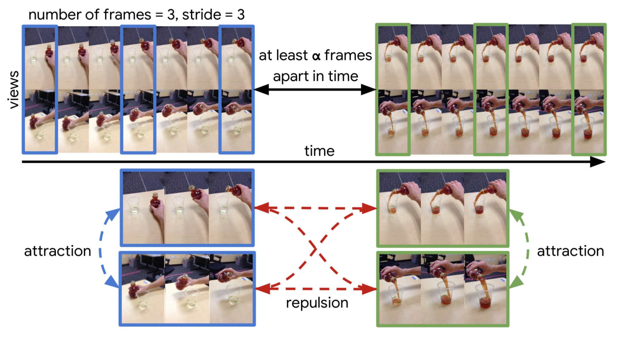
Training data is sampled as follows:

1. Construct two pairs of video clips. Each pair contains two clips from different camera views but synchronized in time. The two clip pairs should be well separated in time.
2. From each clip in a pair, sample a fixed number of frames simultaneously using the same stride.
3. Frames aligned at the same timesteps are treated as positives in the n-pair loss; frames from different pairs serve as negatives.

mfTCN embeddings can encode object position and velocity in a scene (for example, in cartpole), and they can also be used as policy inputs.

Autonomous Goal Generation

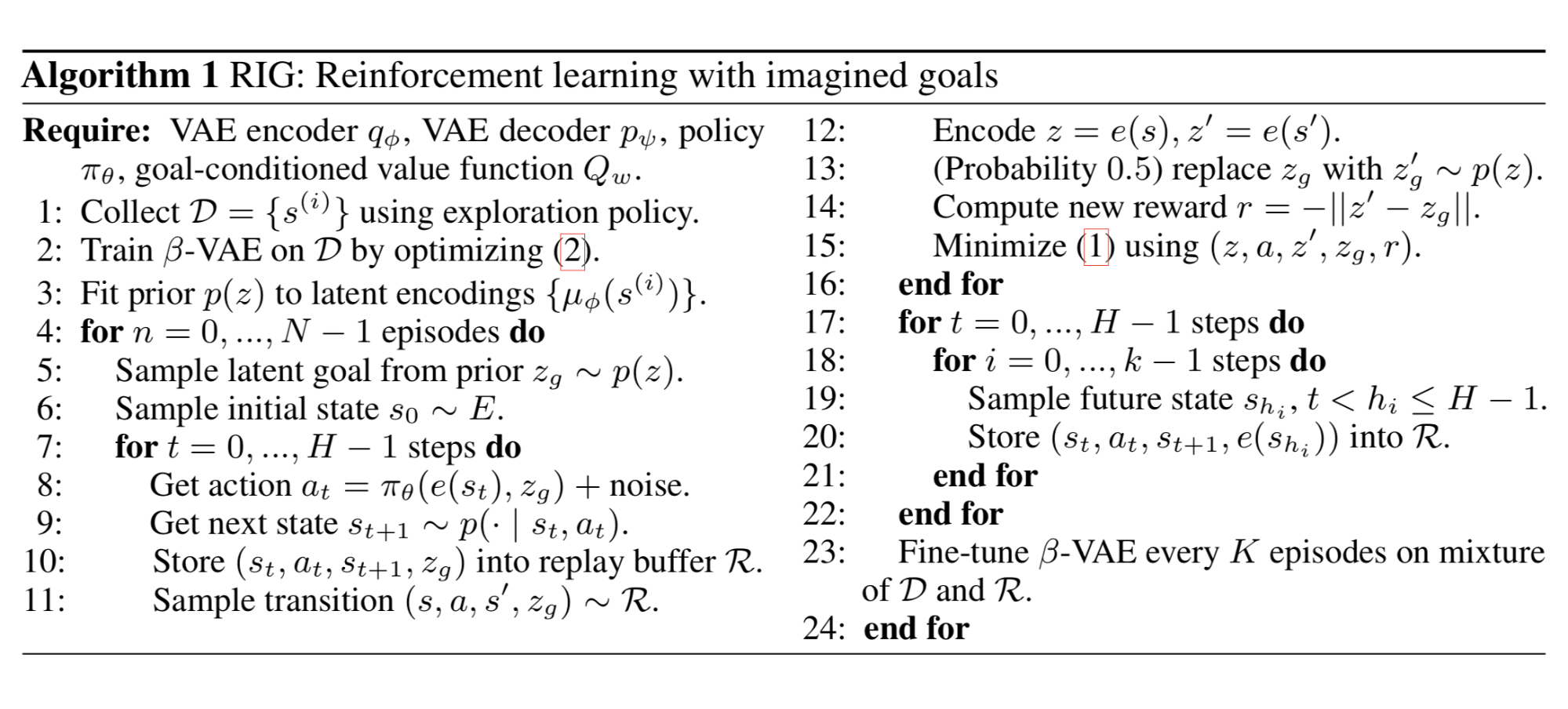
RIG (Reinforcement learning with Imagined Goals; Nair et al., 2018) describes a method for training a goal-conditioned policy using unsupervised representation learning. The policy learns through self-supervised practice by first imagining “fake” goals, then attempting to achieve them.

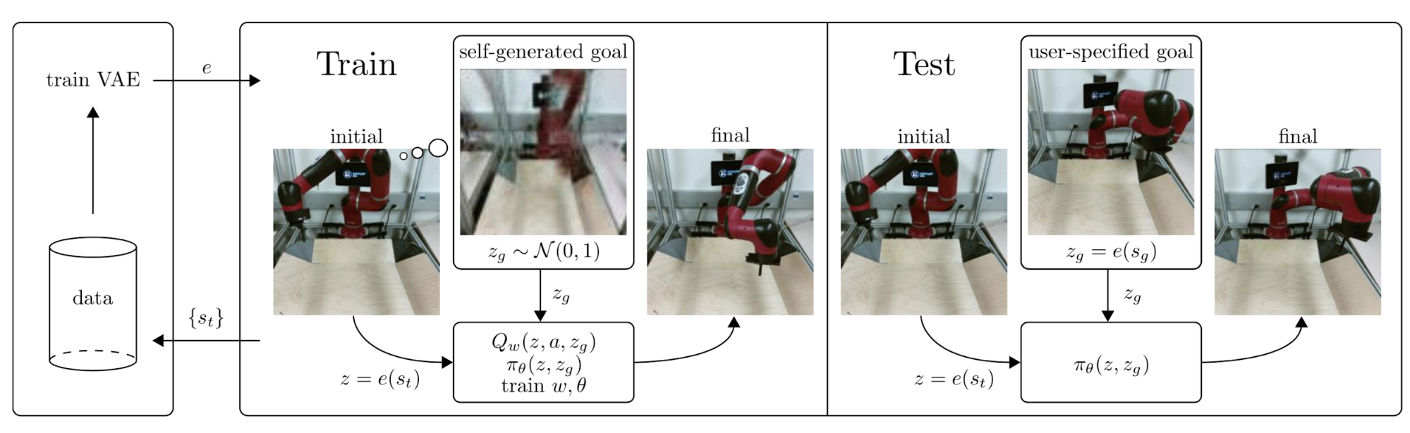
The task is to control a robot arm that pushes a small puck on a table to a desired location. The desired location (the goal) is specified by an image. During training, the method learns latent embeddings for the state $s$ and the goal $g$ using a $\beta$-VAE encoder, and the control policy operates entirely in latent space.

Assume a $\beta$-VAE with encoder $q_\phi$ that maps input states to a latent variable $z$ modeled as a Gaussian distribution, and decoder $p_\psi$ that maps $z$ back to states. In RIG, the state encoder is set to the mean of the $\beta$-VAE encoder:

The reward is defined as the Euclidean distance between the embedded state and goal vectors, $r(s, g) = -|e(s) - e(g)|$. As in grasp2vec, RIG also uses data augmentation via latent goal relabeling: specifically, half of the goals are sampled randomly from the prior, and the other half are chosen using HER. Also as in grasp2vec, the reward depends only on the learned state encoding and not on any ground-truth state, enabling training on real robots.

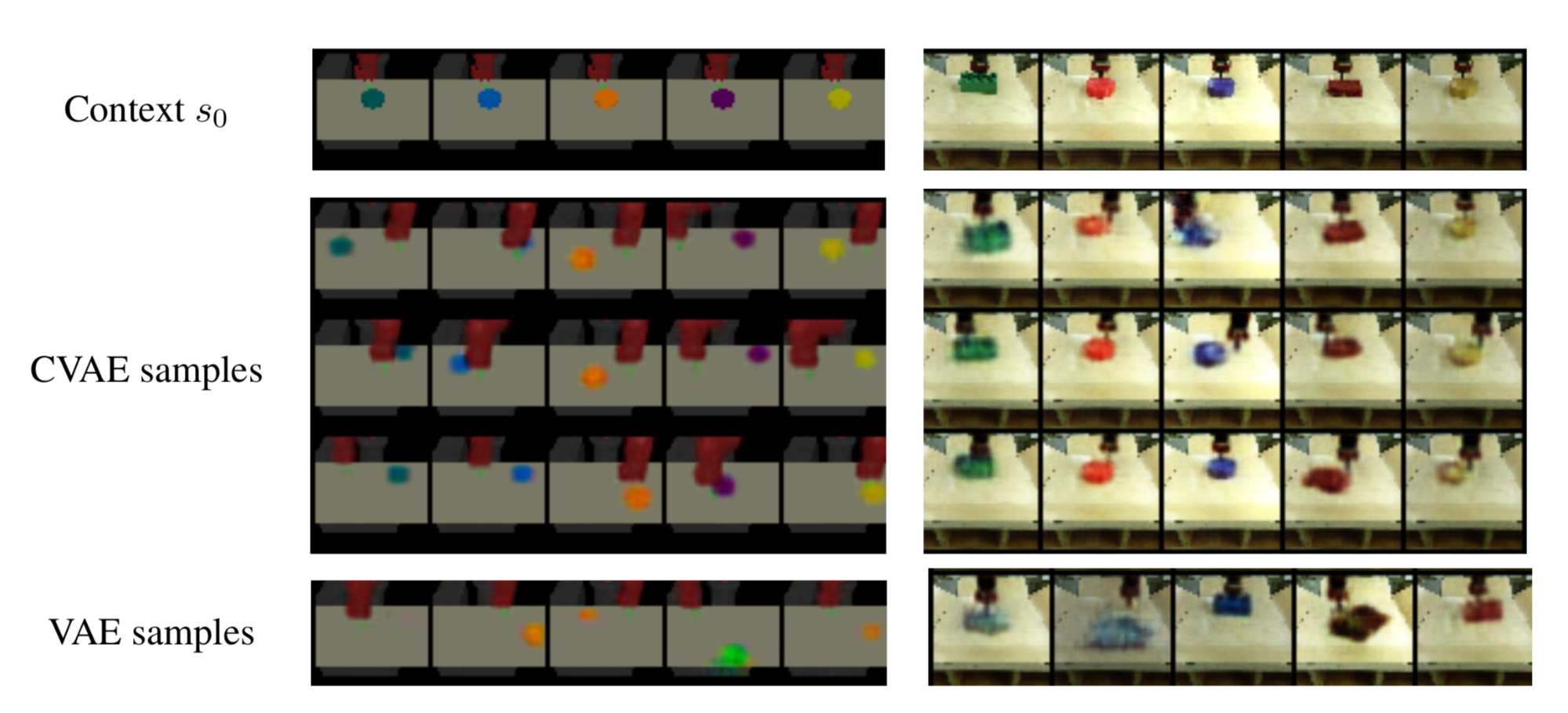
A limitation of RIG is insufficient object diversity in imagined goal images. If $\beta$-VAE is trained only on a black puck, it cannot generate goals involving other objects, such as blocks with different shapes and colors. A subsequent improvement replaces $\beta$-VAE with a CC-VAE (Context-Conditioned VAE; Nair, et al., 2019), inspired by CVAE (Conditional VAE; Sohn, Lee & Yan, 2015), for goal generation.

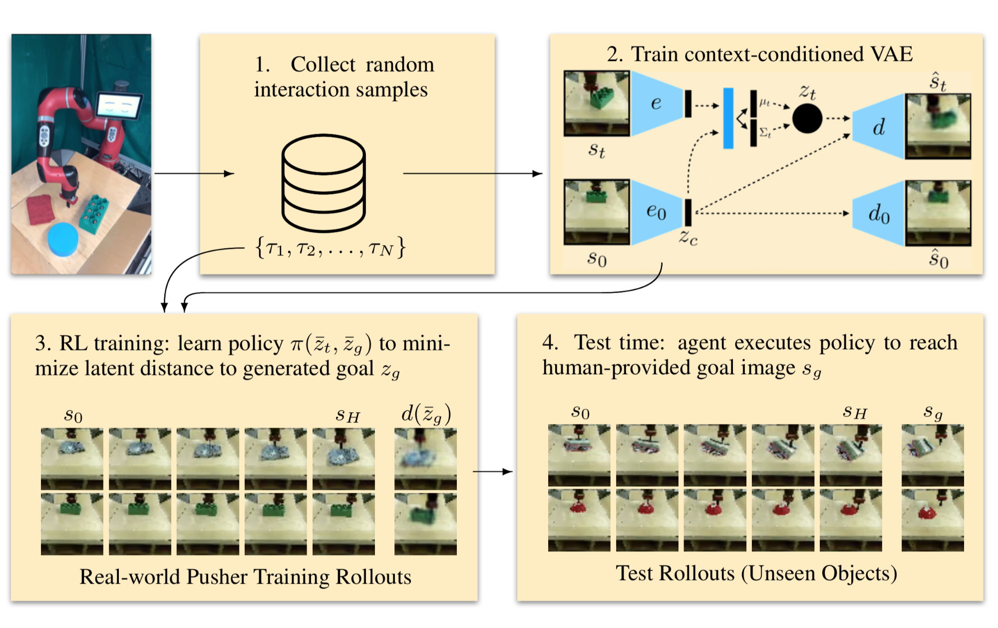
A CVAE conditions on a context variable $c$. It trains an encoder $q_\phi(z \vert s, c)$ and a decoder $p_\psi (s \vert z, c)$, and both are given access to $c$. The CVAE objective penalizes information flow from the input state $s$ through a bottleneck, while allowing unrestricted information flow from $c$ to both the encoder and the decoder.

To generate plausible goals, CC-VAE conditions on a starting state $s_0$ so that the generated goal contains an object type consistent with $s_0$. This consistency is important, for example, if the current scene contains a red puck but the goal image shows a blue block, the policy may be confused.

In addition to the state encoder $e(s) \triangleq \mu_\phi(s)$, CC-VAE trains a second convolutional encoder $e_0(.)$ that maps the starting state $s_0$ into a compact context representation $c = e_0(s_0)$. The two encoders, $e(.)$ and $e_0(.)$, are deliberately distinct and do not share weights, because they are intended to encode different sources of variation in the images. Beyond the standard CVAE loss, CC-VAE adds an additional reconstruction term to recover $c$ from $s_0$, $\hat{s}_0 = d_0(c)$.

Bisimulation

Task-agnostic representations (for example, a model designed to capture all system dynamics) can hinder RL algorithms because they also encode information that is irrelevant to the control objective. For instance, training an autoencoder purely to reconstruct an input image does not guarantee that the resulting representation will be useful for RL. If the goal is to learn only control-relevant information, then reconstruction-based representation learning is often a poor fit because details that do not matter for control can still be essential for accurate reconstruction.

In contrast, bisimulation-based representation learning for control does not rely on reconstruction. Instead, it seeks to cluster states according to their behavioral similarity within an MDP.

Bisimulation (Givan et al. 2003) is an equivalence relation over states that exhibit similar long-term behavior. Bisimulation metrics quantify this relationship, enabling state aggregation that compresses a high-dimensional state space into a smaller one for more efficient computation. The bisimulation distance between two states indicates how behaviorally different those states are.

Given a MDP $\mathcal{M} = \langle \mathcal{S}, \mathcal{A}, \mathcal{P}, \mathcal{R}, \gamma \rangle$ and a bisimulation relation $B$, two states that are equal under relation $B$ (that is, $s_i B s_j$) must share the same immediate reward for every action and have identical transition probabilities over the next bisimilar states:

where $\mathcal{S}_B$ is a partition of the state space induced by the relation $B$.

Note that $=$ is always a bisimulation relation. The most informative choice is the maximal bisimulation relation $\sim$, which induces a partition $\mathcal{S}_\sim$ with the fewest state groups.

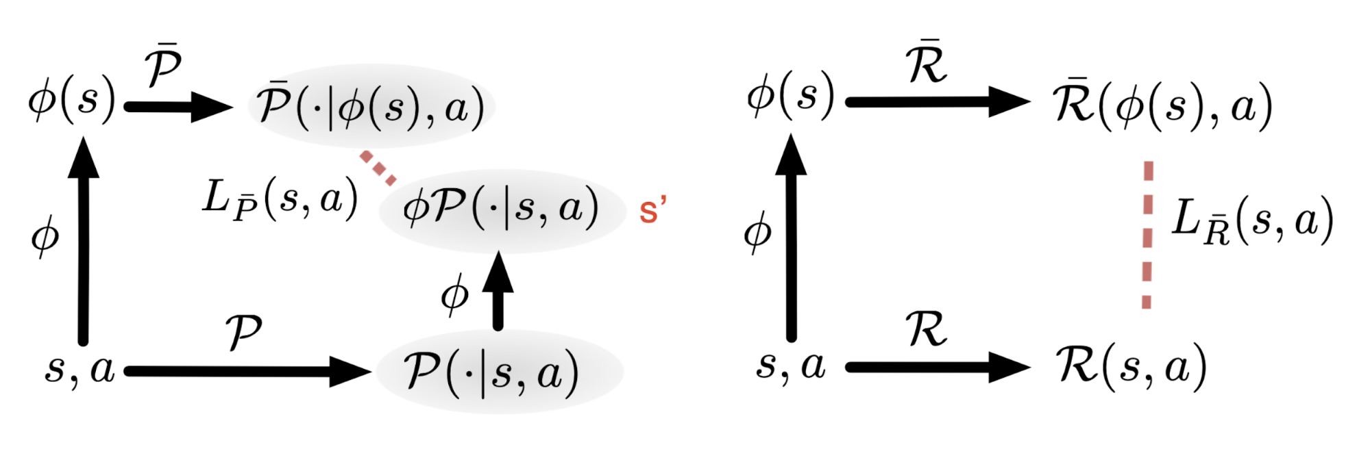
Motivated by an objective similar to that of bisimulation metrics, DeepMDP (Gelada, et al. 2019) reduces high-dimensional observations in RL tasks and learns a latent-space model by minimizing two losses:

1. reward prediction, and
2. prediction of the distribution over the next latent states.

where $\phi(s)$ is the embedding of state $s$. Symbols with bars denote functions (reward function $R$ and transition function $P$) defined on the same MDP but operating within the low-dimensional latent observation space. The embedding representation $\phi$ can be related to bisimulation metrics, because the bisimulation distance is proven to be upper-bounded by the L2 distance in the latent space.

The function $D$ measures the distance between two probability distributions and must be selected with care. DeepMDP emphasizes the Wasserstein-1 metric (also known as “earth-mover distance”). The Wasserstein-1 distance between distributions $P$ and $Q$ on a metric space $(M, d)$ (that is, $d: M \times M \to \mathbb{R}$) is:

where $\Pi(P, Q)$ is the set of all couplings of $P$ and $Q$. $d(x, y)$ specifies the cost of transporting a particle from point $x$ to point $y$.

The Wasserstein metric admits a dual formulation via the Monge-Kantorovich duality:

where $\mathcal{F}_d$ is the set of 1-Lipschitz functions under the metric $d$ - $\mathcal{F}_d = \{ f: \vert f(x) - f(y) \vert \leq d(x, y) \}$.

DeepMDP further generalizes the approach to Norm Maximum Mean Discrepancy (Norm-MMD) metrics to tighten the bounds associated with its deep value function while also reducing computation (Wasserstein is computationally expensive). In their experiments, they observed that the architecture of the transition prediction model can substantially affect performance. When these DeepMDP losses are added as auxiliary objectives while training model-free RL agents, they produce strong improvements on most Atari games.

Deep Bisimulatioin for Control (short for DBC; Zhang et al. 2020) learns latent representations of observations that support effective control in RL tasks, without requiring domain knowledge or pixel-level reconstruction.

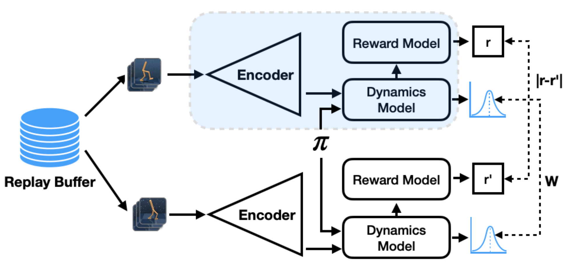
As in DeepMDP, DBC models system dynamics by learning a reward model and a transition model. Both models operate in the latent space, $\phi(s)$. Optimizing the embedding $\phi$ relies on a key result from Ferns, et al. 2004 (Theorem 4.5) and Ferns, et al 2011 (Theorem 2.6):

Given $c \in (0, 1)$ a discounting factor, $\pi$ a policy that is being improved continuously, and $M$ the space of bounded pseudometric on the state space $\mathcal{S}$, we can define $\mathcal{F}: M \mapsto M$:

$ \mathcal{F}(d; \pi)(s_i, s_j) = (1-c) \vert \mathcal{R}_{s_i}^\pi - \mathcal{R}_{s_j}^\pi \vert + c W_d (\mathcal{P}_{s_i}^\pi, \mathcal{P}_{s_j}^\pi) $

Then, $\mathcal{F}$ has a unique fixed point $\tilde{d}$ which is a $\pi^*$-bisimulation metric and $\tilde{d}(s_i, s_j) = 0 \iff s_i \sim s_j$.

[The proof is not trivial. I may or may not add it in the future _(:3」∠)_ …]

Given batches of paired observations, the training loss for $\phi$, $J(\phi)$ minimizes the mean squared error between the on-policy bisimulation metric and the Euclidean distance in the latent space:

where $\bar{\phi}(s)$ denotes $\phi(s)$ with stop gradient, and $\bar{\pi}$ is the mean policy output. The learned reward model $\hat{\mathcal{R}}$ is deterministic, and the learned forward dynamics model $\hat{\mathcal{P}}$ outputs a Gaussian distribution.

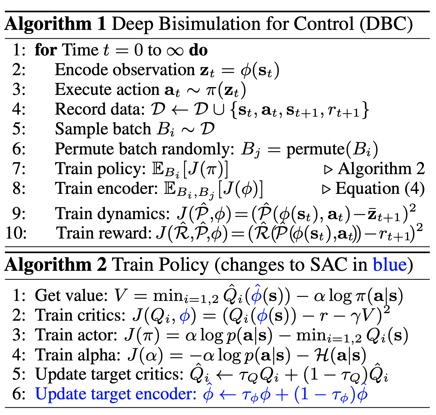
DBC is built on SAC, but it operates in the latent space:

Cited as:

@article{weng2019selfsup,
  title   = "Self-Supervised Representation Learning",
  author  = "Weng, Lilian",
  journal = "lilianweng.github.io",
  year    = "2019",
  url     = "https://lilianweng.github.io/posts/2019-11-10-self-supervised/"
}

References

[1] Alexey Dosovitskiy, et al. “Discriminative unsupervised feature learning with exemplar convolutional neural networks.” IEEE transactions on pattern analysis and machine intelligence 38.9 (2015): 1734-1747.

[2] Spyros Gidaris, Praveer Singh & Nikos Komodakis. “Unsupervised Representation Learning by Predicting Image Rotations” ICLR 2018.

[3] Carl Doersch, Abhinav Gupta, and Alexei A. Efros. “Unsupervised visual representation learning by context prediction.” ICCV. 2015.

[4] Mehdi Noroozi & Paolo Favaro. “Unsupervised learning of visual representations by solving jigsaw puzzles.” ECCV, 2016.

[5] Mehdi Noroozi, Hamed Pirsiavash, and Paolo Favaro. “Representation learning by learning to count.” ICCV. 2017.

[6] Richard Zhang, Phillip Isola & Alexei A. Efros. “Colorful image colorization.” ECCV, 2016.

[7] Pascal Vincent, et al. “Extracting and composing robust features with denoising autoencoders.” ICML, 2008.

[8] Jeff Donahue, Philipp Krähenbühl, and Trevor Darrell. “Adversarial feature learning.” ICLR 2017.

[9] Deepak Pathak, et al. “Context encoders: Feature learning by inpainting.” CVPR. 2016.

[10] Richard Zhang, Phillip Isola, and Alexei A. Efros. “Split-brain autoencoders: Unsupervised learning by cross-channel prediction.” CVPR. 2017.

[11] Xiaolong Wang & Abhinav Gupta. “Unsupervised Learning of Visual Representations using Videos.” ICCV. 2015.

[12] Carl Vondrick, et al. “Tracking Emerges by Colorizing Videos” ECCV. 2018.

[13] Ishan Misra, C. Lawrence Zitnick, and Martial Hebert. “Shuffle and learn: unsupervised learning using temporal order verification.” ECCV. 2016.

[14] Basura Fernando, et al. “Self-Supervised Video Representation Learning With Odd-One-Out Networks” CVPR. 2017.

[15] Donglai Wei, et al. “Learning and Using the Arrow of Time” CVPR. 2018.

[16] Florian Schroff, Dmitry Kalenichenko and James Philbin. “FaceNet: A Unified Embedding for Face Recognition and Clustering” CVPR. 2015.

[17] Pierre Sermanet, et al. “Time-Contrastive Networks: Self-Supervised Learning from Video” CVPR. 2018.

[18] Debidatta Dwibedi, et al. “Learning actionable representations from visual observations.” IROS. 2018.

[19] Eric Jang & Coline Devin, et al. “Grasp2Vec: Learning Object Representations from Self-Supervised Grasping” CoRL. 2018.

[20] Ashvin Nair, et al. “Visual reinforcement learning with imagined goals” NeuriPS. 2018.

[21] Ashvin Nair, et al. “Contextual imagined goals for self-supervised robotic learning” CoRL. 2019.

[22] Aaron van den Oord, Yazhe Li & Oriol Vinyals. “Representation Learning with Contrastive Predictive Coding” arXiv preprint arXiv:1807.03748, 2018.

[23] Olivier J. Henaff, et al. “Data-Efficient Image Recognition with Contrastive Predictive Coding” arXiv preprint arXiv:1905.09272, 2019.

[24] Kaiming He, et al. “Momentum Contrast for Unsupervised Visual Representation Learning.” CVPR 2020.

[25] Zhirong Wu, et al. “Unsupervised Feature Learning via Non-Parametric Instance-level Discrimination.” CVPR 2018.

[26] Ting Chen, et al. “A Simple Framework for Contrastive Learning of Visual Representations.” arXiv preprint arXiv:2002.05709, 2020.

[27] Aravind Srinivas, Michael Laskin & Pieter Abbeel “CURL: Contrastive Unsupervised Representations for Reinforcement Learning.” arXiv preprint arXiv:2004.04136, 2020.

[28] Carles Gelada, et al. “DeepMDP: Learning Continuous Latent Space Models for Representation Learning” ICML 2019.

[29] Amy Zhang, et al. “Learning Invariant Representations for Reinforcement Learning without Reconstruction” arXiv preprint arXiv:2006.10742, 2020.

[30] Xinlei Chen, et al. “Improved Baselines with Momentum Contrastive Learning” arXiv preprint arXiv:2003.04297, 2020.

[31] Jean-Bastien Grill, et al. “Bootstrap Your Own Latent: A New Approach to Self-Supervised Learning” arXiv preprint arXiv:2006.07733, 2020.

[32] Abe Fetterman & Josh Albrecht. “Understanding self-supervised and contrastive learning with Bootstrap Your Own Latent (BYOL)” Untitled blog. Aug 24, 2020.