Exploitation versus exploration is a foundational concern in reinforcement learning. This post describes several widely used methods for improving exploration in Deep RL.

[Updated on 2020-06-17: Add “exploration via disagreement” in the “Forward Dynamics” section.

Exploitation versus exploration is a central theme in Reinforcement Learning. Ideally, an RL agent should identify an optimal solution as quickly as possible. At the same time, locking into choices too early, without sufficient exploration, is risky because it can result in local minima or even complete failure. Modern RL algorithms that directly optimize for high return often achieve efficient exploitation, whereas effective exploration remains comparatively less resolved.

This article reviews several common exploration strategies used in Deep RL. The space is broad, and this post does not attempt to cover every important subtopic. I intend to update it over time and gradually expand the material.

Classic Exploration Strategies

As a brief refresher, we begin with several classic exploration algorithms that work well for multi-armed bandits or simple tabular RL.

• Epsilon-greedy: The agent performs random exploration occasionally with probability $\epsilon$, and selects the optimal action most of the time with probability $1-\epsilon$.
• Upper confidence bounds: The agent chooses the greedy action that maximizes the upper confidence bound $\hat{Q}_t(a) + \hat{U}_t(a)$, where $\hat{Q}_t(a)$ is the average reward associated with action $a$ up to time $t$, and $\hat{U}_t(a)$ is a function inversely proportional to the number of times action $a$ has been selected. For details, see here.
• Boltzmann exploration: The agent samples actions from a boltzmann distribution (softmax) over learned Q values, controlled by a temperature parameter $\tau$.
• Thompson sampling: The agent maintains a belief over which actions are optimal and samples from that belief distribution. For details, see here.

The following approaches are commonly used to improve exploration during deep RL training, where neural networks serve as function approximators:

• Entropy loss term: Add an entropy term $H(\pi(a \vert s))$ to the loss function, encouraging the policy to select a more diverse set of actions.
• Noise-based Exploration: Inject noise into the observation space, action space, or even the parameter space (Fortunato, et al. 2017, Plappert, et al. 2017).

Key Exploration Problems

Exploration becomes particularly challenging when rewards are rare (providing minimal feedback) or when the environment contains distracting noise. Many exploration methods are designed to address one or both of the following issues.

The Hard-Exploration Problem

The “hard-exploration” problem describes exploration in environments with extremely sparse, or even deceptive, rewards. In these settings, random exploration is unlikely to reach successful states or to generate informative feedback.

Montezuma’s Revenge is a concrete example of the hard-exploration problem. It remains one of the challenging Atari games for DRL, and it is frequently used as a benchmark across papers.

The Noisy-TV Problem

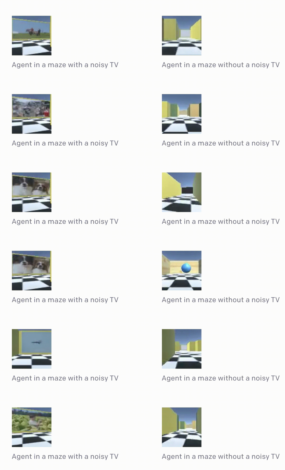
The “Noisy-TV” problem was introduced as a thought experiment in Burda, et al (2018). Consider an RL agent rewarded for seeking novel experiences. A television that outputs uncontrollable and unpredictable random noise could continually attract the agent, indefinitely. The agent keeps receiving novelty rewards from the noisy TV, but it makes no meaningful progress and effectively becomes a “couch potato”.

Intrinsic Rewards as Exploration Bonuses

A common way to improve exploration, particularly for the hard-exploration setting, is to augment the environment reward with an additional bonus signal that explicitly promotes exploration. The policy is then trained using a reward with two components, $r_t = r^e_t + \beta r^i_t$, where $\beta$ is a hyperparameter that controls the tradeoff between exploitation and exploration.

• $r^e_t$ is the extrinsic environment reward at time $t$, defined by the task objective.
• $r^i_t$ is the intrinsic exploration bonus at time $t$.

This intrinsic reward framing is loosely motivated by intrinsic motivation in psychology (Oudeyer & Kaplan, 2008). Curiosity-driven exploration may be a key mechanism by which children develop and learn. Put differently, exploratory behavior can be intrinsically rewarding in the human mind, which helps sustain it. In an RL setting, intrinsic rewards may be tied to curiosity, surprise, state familiarity, and many other signals.

The same principles can be applied in RL algorithms. In the sections below, bonus-based intrinsic rewards are grouped into two broad categories:

1. Discovering novel states
2. Improving the agent’s knowledge of the environment.

Count-based Exploration

If intrinsic rewards reflect what is surprising, then we need a mechanism to assess whether a state is novel or frequently encountered. A direct and intuitive approach is to count how often each state has been visited and assign a bonus accordingly. The bonus encourages policies that prefer rarely visited states over commonly visited states. This is the count-based exploration approach.

Let $N_n(s)$ denote the empirical count function that records the true number of visits to a state $s$ within the sequence $s_{1:n}$. Unfortunately, applying $N_n(s)$ directly is not practical because most states would have $N_n(s)=0$, especially when the state space is continuous or high-dimensional. What is needed is a non-zero count estimate for most states, including those not previously observed.

Counting by Density Model

Bellemare, et al. (2016) proposed using a density model to approximate state visitation frequency, along with a method to derive a pseudo-count from that model. First, define a conditional probability over the state space, $\rho_n(s) = \rho(s \vert s_{1:n})$, as the probability that the $(n+1)$-th state equals $s$ given that the first $n$ states are $s_{1:n}$. Empirically, this can be estimated with $N_n(s)/n$.

Next, define the recoding probability of a state $s$ as the probability the density model assigns to $s$ after observing one additional occurrence of $s$, $\rho’_n(s) = \rho(s \vert s_{1:n}s)$.

The paper introduced two quantities to regulate the density model more effectively: a pseudo-count function $\hat{N}_n(s)$ and a pseudo-count total $\hat{n}$. Because these are intended to imitate empirical counts, we should have:

The relationship between $\rho_n(x)$ and $\rho’_n(x)$ requires the density model to be learning-positive: for all $s_{1:n} \in \mathcal{S}^n$ and all $s \in \mathcal{S}$, $\rho_n(s) \leq \rho’_n(s)$. That is, after observing one instance of $s$, the model’s predicted probability for that same $s$ should increase. In addition to being learning-positive, the density model must be trained fully online using non-randomized mini-batches of experienced states, and therefore we naturally have $\rho’_n = \rho_{n+1}$.

The pseudo-count can be computed from $\rho_n(s)$ and $\rho’_n(s)$ by solving the linear system above:

Alternatively, it can be estimated using the prediction gain (PG):

A common form for count-based intrinsic bonuses is $r^i_t = N(s_t, a_t)^{-1/2}$ (as in MBIE-EB; Strehl & Littman, 2008). The pseudo-count exploration bonus follows an analogous shape, $r^i_t = \big(\hat{N}_n(s_t, a_t) + 0.01 \big)^{-1/2}$.

In Bellemare et al., (2016), experiments used a simple CTS (Context Tree Switching) density model to estimate pseudo-counts. CTS takes a 2D image as input and assigns a probability based on the product of location-dependent L-shaped filters, where each filter’s prediction is produced by a CTS algorithm trained on prior images. Although straightforward, CTS is constrained in expressiveness, scalability, and data efficiency. In later work, Georg Ostrovski, et al. (2017) improved the method by training a PixelCNN (van den Oord et al., 2016) as the density model.

As another option, the density model may be a Gaussian Mixture Model, as in Zhao & Tresp (2018). They used a variational GMM to estimate trajectory density (for example, by concatenating a sequence of states), and then used the predicted probabilities to guide prioritization in experience replay in an off-policy setting.

Counting after Hashing

Another approach for enabling counting in high-dimensional state spaces is to map states to hash codes, making state occurrences trackable (Tang et al. 2017). The state space is discretized via a hash function $\phi: \mathcal{S} \mapsto \mathbb{Z}^k$. An exploration bonus $r^{i}: \mathcal{S} \mapsto \mathbb{R}$ is added to the reward, defined as $r^{i}(s) = {N(\phi(s))}^{-1/2}$, where $N(\phi(s))$ is the empirical count of occurrences of $\phi(s)$.

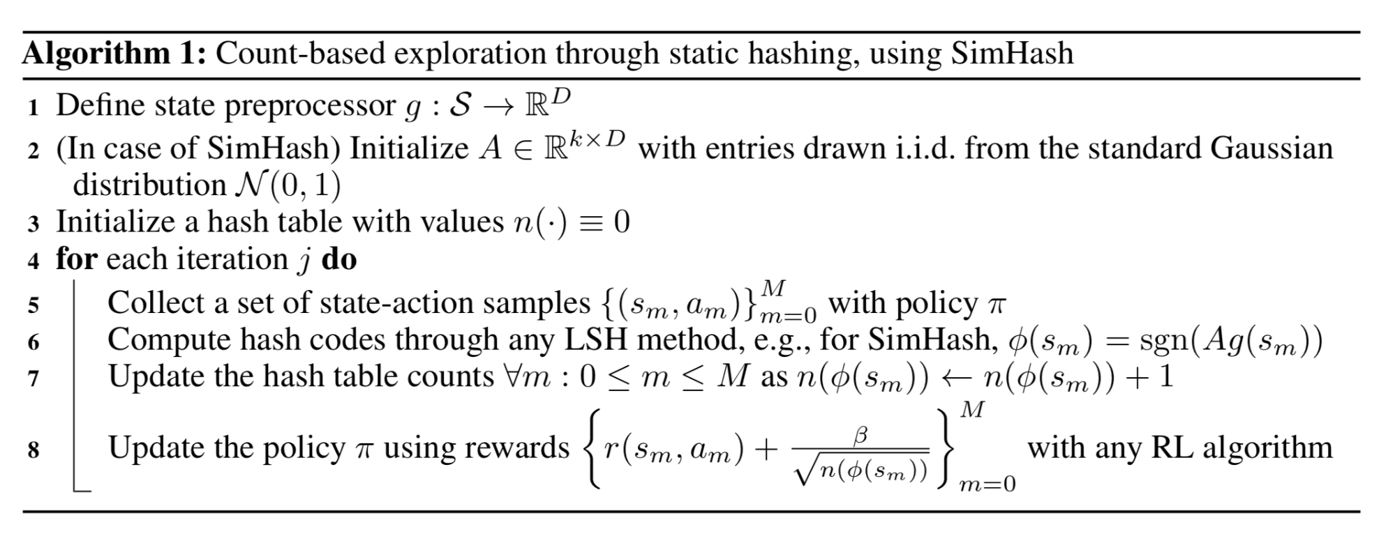
Tang et al. (2017) proposed using Locality-Sensitive Hashing (LSH) to transform continuous, high-dimensional data into discrete hash codes. LSH is a widely used family of hashing methods for nearest-neighbor retrieval under a similarity metric. A hashing scheme $x \mapsto h(x)$ is locality-sensitive if it preserves distance information between data points, such that nearby vectors produce similar hashes while distant vectors produce very different hashes. (For another use of LSH, see Transformer improvement.) SimHash is a computationally efficient LSH variant that measures similarity using angular distance:

where $A \in \mathbb{R}^{k \times D}$ is a matrix whose entries are drawn i.i.d. from a standard Gaussian distribution, and $g: \mathcal{S} \mapsto \mathbb{R}^D$ is an optional preprocessing function. The binary code dimension is $k$, which determines the discretization granularity of the state space. Larger $k$ yields finer granularity and fewer collisions.

For high-dimensional images, SimHash may not perform well when applied directly to raw pixels. To address this, Tang et al. (2017) designed an autoencoder (AE) that takes states $s$ as input and learns hash codes. The AE includes a special dense layer with $k$ sigmoid units as its latent representation. The sigmoid activations $b(s)$ are then binarized by rounding to the nearest binary values $\lfloor b(s)\rceil \in \{0, 1\}^D$, producing the binary hash codes for state $s$. The AE loss over $n$ states has two components:

One limitation of this method is that dissimilar inputs $s_i, s_j$ can map to identical hash codes while still being reconstructed perfectly by the AE. One might consider replacing the bottleneck layer $b(s)$ with explicit hash codes $\lfloor b(s)\rceil$; however, gradients cannot be backpropagated through the rounding operation. Adding uniform noise can reduce this issue because the AE must learn to separate the latent variables more strongly to counteract the injected noise.

Prediction-based Exploration

The second major class of intrinsic exploration bonuses rewards improvements in the agent’s knowledge of the environment. The agent’s familiarity with the environment dynamics can be estimated using a prediction model. Using prediction error as a proxy for curiosity was proposed long ago (Schmidhuber, 1991).

Forward Dynamics

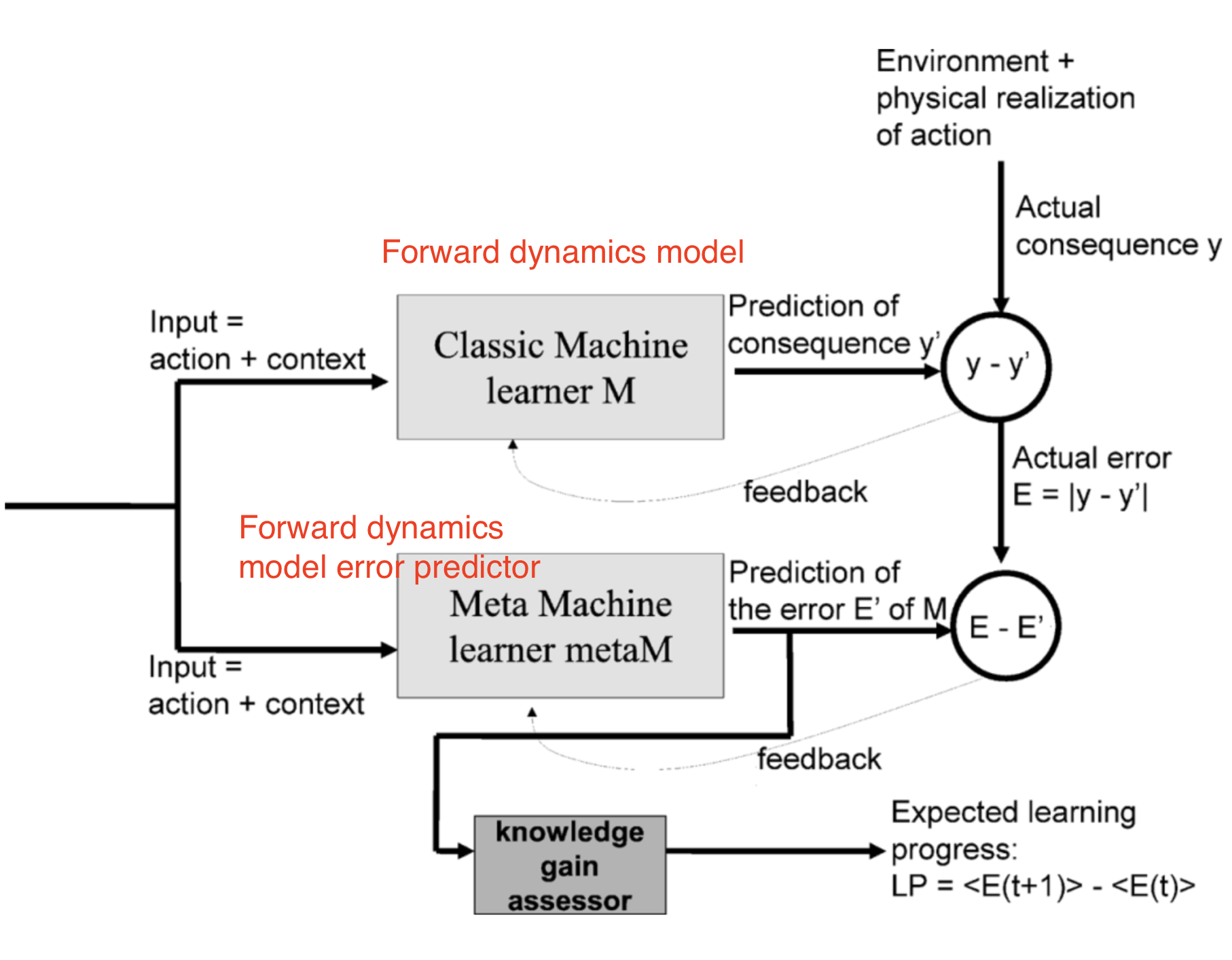
Learning a forward dynamics prediction model provides a practical approximation of how much knowledge the agent has acquired about the environment and the task MDPs. The model captures the agent’s ability to predict the consequences of its behavior, $f: (s_t, a_t) \mapsto s_{t+1}$. Because such a model cannot be perfect (for example, due to partial observability), its error $e(s_t, a_t) = | f(s_t, a_t) - s_{t+1} |^2_2$ can serve as an intrinsic exploration reward. Higher prediction error suggests lower familiarity with the state. Moreover, a faster decline in error indicates greater learning progress and thus a stronger progress signal.

Intelligent Adaptive Curiosity (IAC; Oudeyer, et al. 2007) outlined the use of a forward dynamics predictor to estimate learning progress and to define intrinsic rewards accordingly.

IAC uses a memory storing all experiences encountered by the robot, $M=\{(s_t, a_t, s_{t+1})\}$, together with a forward dynamics model $f$. It incrementally partitions the state space (sensorimotor space in the paper’s robotics setting) into regions based on transition samples, following a procedure analogous to decision-tree splitting. A split occurs when the sample count exceeds a threshold, and the method aims to minimize state variance within each leaf. Each node is defined by its exclusive sample set and maintains its own forward dynamics predictor $f$, referred to as an “expert”.

Each expert’s prediction error $e_t$ is appended to a region-specific list. Learning progress is then computed as the difference between the mean error of a moving window offset by $\tau$ and the mean error of the current moving window. The intrinsic reward is defined to track this learning progress: $r^i_t = \frac{1}{k}\sum_{i=0}^{k-1}(e_{t-i-\tau} - e_{t-i})$, where $k$ is the window size. Thus, the greater the decrease in prediction error, the larger the intrinsic reward assigned to the agent. Equivalently, the agent is encouraged to choose actions that lead to rapid learning about the environment.

Stadie et al. (2015) trained a forward dynamics model in an encoding space defined by $\phi$, $f_\phi: (\phi(s_t), a_t) \mapsto \phi(s_{t+1})$. The prediction error at time $T$ is normalized by the maximum error observed up to time $t$, $\bar{e}_t = \frac{e_t}{\max_{i \leq t} e_i}$, ensuring it stays within [0, 1]. The intrinsic reward is then defined as $r^i_t = (\frac{\bar{e}_t(s_t, a_t)}{t \cdot C})$, where $C > 0$ is a decay constant.

State encoding via $\phi(.)$ is necessary, as the paper’s experiments show that a dynamics model trained directly on raw pixels exhibits very poor behavior, assigning nearly identical exploration bonuses to all states. In Stadie et al. (2015), the encoding function $\phi$ is learned using an autoencoder (AE), and $\phi(.)$ is one of the AE output layers. The AE can be trained offline using images collected by a random agent, or trained online jointly with the policy, where early frames are gathered using $\epsilon$-greedy exploration.

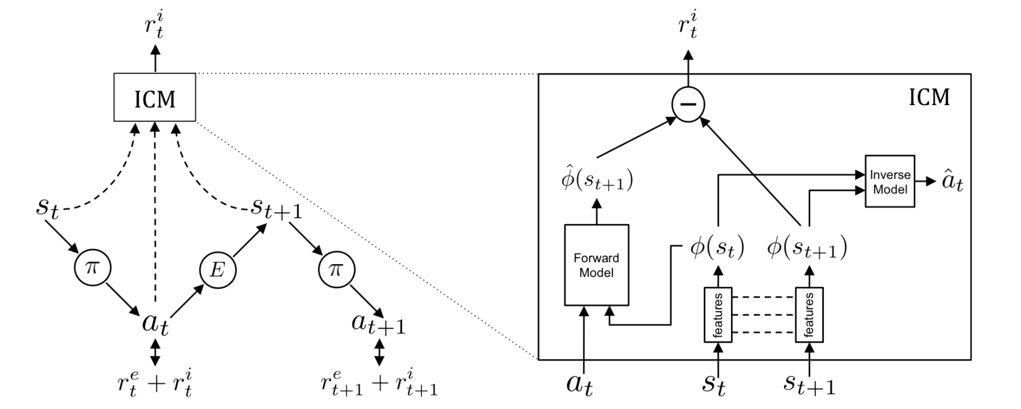
Rather than using an autoencoder, the Intrinsic Curiosity Module (ICM; Pathak, et al., 2017) learns the state encoding $\phi(.)$ using a self-supervised inverse dynamics model. Predicting the next state given the agent’s action can be difficult, particularly because some environmental factors are uncontrollable or irrelevant to the agent’s influence. ICM argues that a useful feature space should exclude such factors because they cannot influence the agent’s behavior and thus the agent has no incentive for learning them. By training an inverse dynamics model $g: (\phi(s_t), \phi(s_{t+1})) \mapsto a_t$, the feature representation focuses on environment changes that are attributable to the agent’s actions and disregards the rest.

Given a forward model $f$, an inverse dynamics model $g$ and an observation $(s_t, a_t, s_{t+1})$:

This $\phi(.)$ is expected to be robust to uncontrollable aspects of the environment.

Burda, Edwards & Pathak, et al. (2018) conducted large-scale comparisons of purely curiosity-driven learning, meaning that the agent receives only intrinsic rewards. In their setup, the reward is $r_t = r^i_t = | f(s_t, a_t) - \phi(s_{t+1})|_2^2$. Selecting $\phi$ is critical for learning forward dynamics; the representation is expected to be compact, sufficient, and stable, making prediction more tractable and filtering out irrelevant observations.

They compared four encoding functions:

1. Raw image pixels: no encoding, $\phi(x) = x$.
2. Random features (RF): each state is compressed by a fixed random neural network.
3. VAE: encoding via a probabilistic encoder, $\phi(x) = q(z \vert x)$.
4. Inverse dynamic features (IDF): the same feature representation used in ICM.

Across all experiments, reward signals are normalized using a running estimate of the standard deviation of cumulative returns. In addition, all experiments use an infinite-horizon setting to prevent the “done” flag from leaking information.

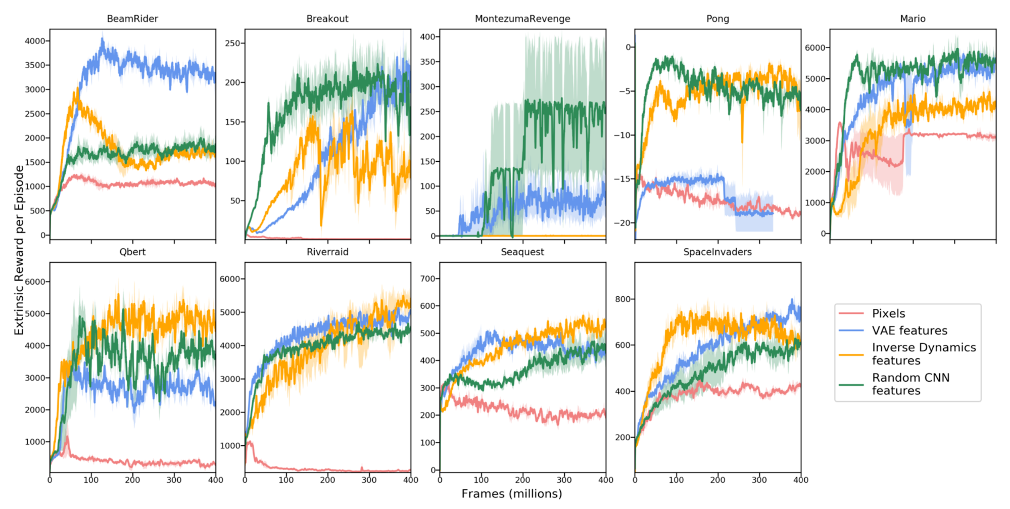
Notably, random features are quite competitive. However, in feature-transfer experiments (training an agent in Super Mario Bros level 1-1 and then testing in another level), learned IDF representations generalize more effectively.

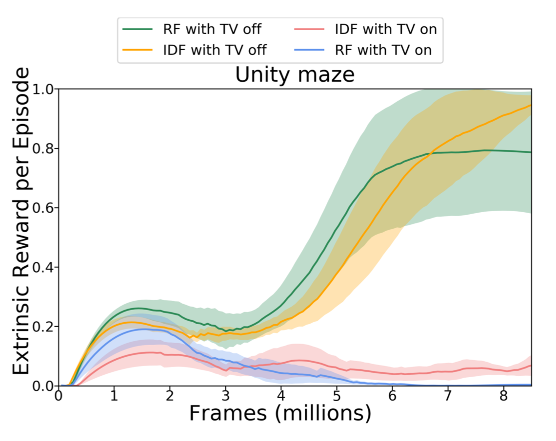
They also evaluated RF and IDF in an environment that includes a noisy TV. As expected, the noisy TV significantly slows learning, and extrinsic rewards remain much lower over time.

Forward dynamics optimization can also be framed through variational inference. VIME (short for “Variational information maximizing exploration”; Houthooft, et al. 2017) is an exploration strategy that maximizes information gain about the agent’s belief over environment dynamics. The amount of newly acquired information about forward dynamics can be quantified as a reduction in entropy.

Let $\mathcal{P}$ be the environment transition function, $p(s_{t+1}\vert s_t, a_t; \theta)$ the forward prediction model parameterized by $\theta \in \Theta$, and $\xi_t = \{s_1, a_1, \dots, s_t\}$ the trajectory history. The goal is to reduce entropy after taking a new action and observing the next state, which corresponds to maximizing:

By taking an expectation over potential next states, the agent is incentivized to choose an action that increases the KL divergence (the “information gain”) between its updated belief about the prediction model and its prior belief. This quantity can be incorporated into the reward as an intrinsic term: $r^i_t = D_\text{KL} [p(\theta \vert \xi_t, a_t, s_{t+1}) | p(\theta \vert \xi_t))]$.

However, computing the posterior $p(\theta \vert \xi_t, a_t, s_{t+1})$ is generally intractable.

Because $p(\theta\vert\xi_t)$ is difficult to compute directly, a natural strategy is to approximate it using an alternative distribution $q_\phi(\theta)$. Using a variational lower bound, maximizing $q_\phi(\theta)$ is equivalent to maximizing $p(\xi_t\vert\theta)$ while minimizing $D_\text{KL}[q_\phi(\theta) | p(\theta)]$.

With approximation distribution $q$, the intrinsic reward becomes:

Here, $\phi_{t+1}$ denotes the parameters of $q$ associated with the updated relief after observing $a_t$ and $s_{t+1}$. When this quantity is used as an exploration bonus, it is normalized by dividing it by the moving median of the corresponding KL divergence value.

In this setting, the dynamics model is parameterized as a Bayesian neural network (BNN), which maintains a distribution over its weights. The BNN weight distribution $q_\phi(\theta)$ is modeled as a fully factorized Gaussian with $\phi = \{\mu, \sigma\}$, enabling straightforward sampling of $\theta \sim q_\phi(.)$. After applying a second-order Taylor expansion, the KL term $D_\text{KL}[q_{\phi + \lambda \Delta\phi}(\theta) | q_{\phi}(\theta)]$ can be approximated using Fisher Information Matrix $\mathbf{F}_\phi$. This computation is efficient because $q_\phi$ is a factorized Gaussian, so its covariance matrix is diagonal. For additional details, see the paper, particularly Sections 2.3 to 2.5.

All of the methods described above rely on a single prediction model. When multiple such models are available, the disagreement among them can be used to define the exploration bonus (Pathak, et al. 2019). Large disagreement reflects low predictive confidence and therefore suggests that additional exploration is needed. Pathak, et al. (2019) proposed training an ensemble of forward dynamics models and using the variance across the ensemble outputs as $r_t^i$. Specifically, they encode the state space with random feature and train 5 models in the ensemble.

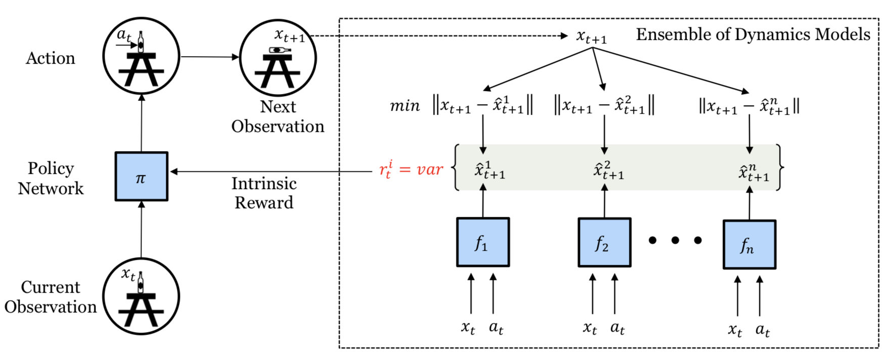
Because $r^i_t$ is differentiable, the intrinsic reward in the model can be optimized directly via gradient descent, allowing it to guide the policy agent toward action changes. This differentiable exploration method is highly efficient, but it is constrained by a short exploration horizon.

Random Networks

What happens if the prediction task is not related to environment dynamics at all? In practice, prediction on a random task can still promote effective exploration.

DORA (short for “Directed Outreaching Reinforcement Action-Selection”; Fox & Choshen, et al. 2018) is a framework that injects exploration signals through a newly introduced, task-independent MDP. DORA is based on two parallel MDPs:

• The original task MDP.
• An identical MDP but with no reward attached. Instead, every state-action pair is constructed to have value 0. The Q-value learned for this second MDP is referred to as the E-value. If the model cannot perfectly predict the E-value as zero, then it is still lacking information.

At initialization, the E-value is set to 1. This positive initialization encourages directed exploration that improves E-value prediction. State-action pairs with high estimated E-values indicate insufficient information has been collected so far, at least not enough to rule out those high E-values. In this sense, the logarithm of E-values can be viewed as a generalization of visit counters.

When neural networks are used for function approximation of the E-value, an additional value head is introduced to predict the E-value, and it is simply trained to output zero. Given a predicted E-value $E(s_t, a_t)$, the exploration bonus is $r^i_t = \frac{1}{\sqrt{-\log E(s_t, a_t)}}$.

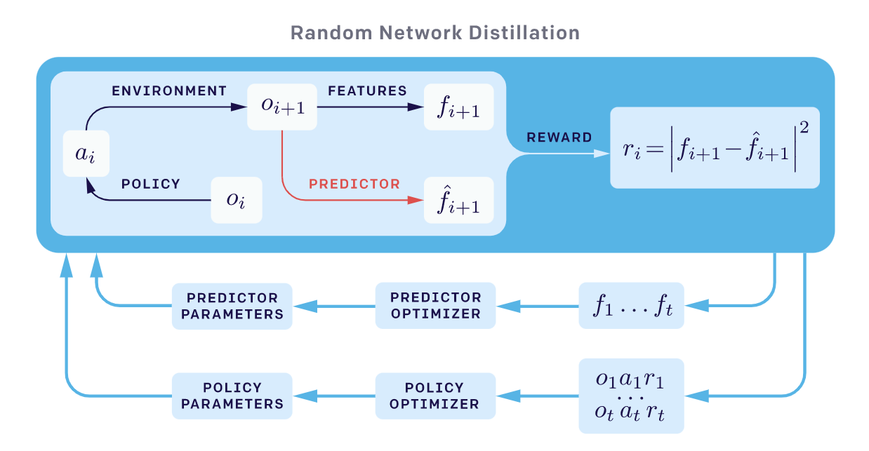
In a similar spirit, Random Network Distillation (RND; Burda, et al. 2018) defines a prediction task that is independent of the main task. The RND exploration bonus is the prediction error of a neural network $\hat{f}(s_t)$ that attempts to match features of observations produced by a fixed randomly initialized neural network $f(s_t)$. The intuition is that, for a newly encountered state, if similar states have been visited frequently in the past, the prediction task becomes easier and the error decreases. The exploration bonus is $r^i(s_t) = |\hat{f}(s_t; \theta) - f(s_t) |_2^2$.

Two considerations are critical in RND experiments:

1. A non-episodic setting yields stronger exploration, particularly when no extrinsic rewards are provided. In this setting, the return is not truncated at “Game over”, and intrinsic return can propagate across multiple episodes.
2. Normalization matters, because the reward scale is difficult to tune when a random neural network serves as the prediction target. The intrinsic reward is normalized by dividing by a running estimate of the standard deviation of the intrinsic return.

This RND configuration performs well on hard-exploration tasks. For example, maximizing the RND exploration bonus consistently discovers more than half of the rooms in Montezuma’s Revenge.

Physical Properties

Unlike games in simulators, certain RL applications, such as robotics, must understand objects and perform intuitive physical reasoning. Some prediction tasks require the agent to execute a sequence of interactions and observe the resulting consequences, for example, to estimate hidden physical properties (such as mass, friction, and so on).

Motivated by these considerations, Denil, et al. (2017) showed that DRL agents can learn to perform the exploration required to uncover such hidden properties. They studied two experiments:

1. “Which is heavier?” The agent must interact with blocks and infer which block is heavier.
2. “Towers” The agent must infer how many rigid bodies make up a tower by knocking it down.

In these experiments, the agent first enters an exploration phase, during which it interacts with the environment to gather information. After the exploration phase ends, the agent must output a labeling action to answer the question. A positive reward is given if the answer is correct; otherwise, a negative reward is given. Because answering requires substantial interaction with objects in the scene, the agent must learn to explore efficiently in order to infer the underlying physics and select the correct answer. Exploration therefore emerges naturally.

In their results, the agent learns both tasks, with performance varying by task difficulty. Although the work does not use the physics prediction task as an intrinsic reward bonus in combination with extrinsic rewards for a separate learning objective, it instead focuses on the exploration tasks themselves. I appreciate the idea of encouraging sophisticated exploration behavior through prediction of hidden physical properties in the environment.

Memory-based Exploration

Reward-based exploration has several limitations:

• Function approximation adapts slowly.
• The exploration bonus is non-stationary.
• Knowledge fading, meaning states stop being novel and therefore fail to deliver intrinsic reward signals quickly enough.

The methods in this section use external memory to address the weaknesses of reward bonus-based exploration.

Episodic Memory

As noted earlier, RND performs better in a non-episodic setting, where predictive knowledge accumulates across episodes. The exploration strategy Never Give Up (NGU; Badia, et al. 2020a) combines an episodic novelty module, which adapts quickly within a single episode, with RND as a lifelong novelty module.

Concretely, NGU defines intrinsic reward as the combination of two exploration bonuses, one computed within a single episode and one computed across multiple episodes.

The short-term, per-episode reward is produced by an episodic novelty module. This module includes an episodic memory $M$ (a dynamically sized, slot-based memory) and an IDF (inverse dynamics features) embedding function $\phi$, which matches the feature encoding used in ICM.

1. At each time step, the current state embedding $\phi(s_t)$ is added to $M$.

2. The intrinsic bonus is computed by comparing the current observation with the contents of $M$. Greater dissimilarity yields a larger bonus.

   $ r^\text{episodic}_t \approx \frac{1}{\sqrt{\sum_{\phi_i \in N_k} K(\phi(x_t), \phi_i)} + c} $

   Here, $K(x, y)$ is a kernel function that measures the distance between two samples. $N_k$ denotes a set of $k$ nearest neighbors in $M$ according to $K(., .)$. $c$ is a small constant that prevents the denominator from becoming zero. In the paper, $K(x, y)$ is set as the inverse kernel:

   $ K(x, y) = \frac{\epsilon}{\frac{d^2(x, y)}{d^2_m} + \epsilon} $

   where $d(.,.)$ is the Euclidean distance between two samples, and $d_m$ is a running average of the squared Euclidean distance of the k-th nearest neighbors to improve robustness. $\epsilon$ is a small constant.

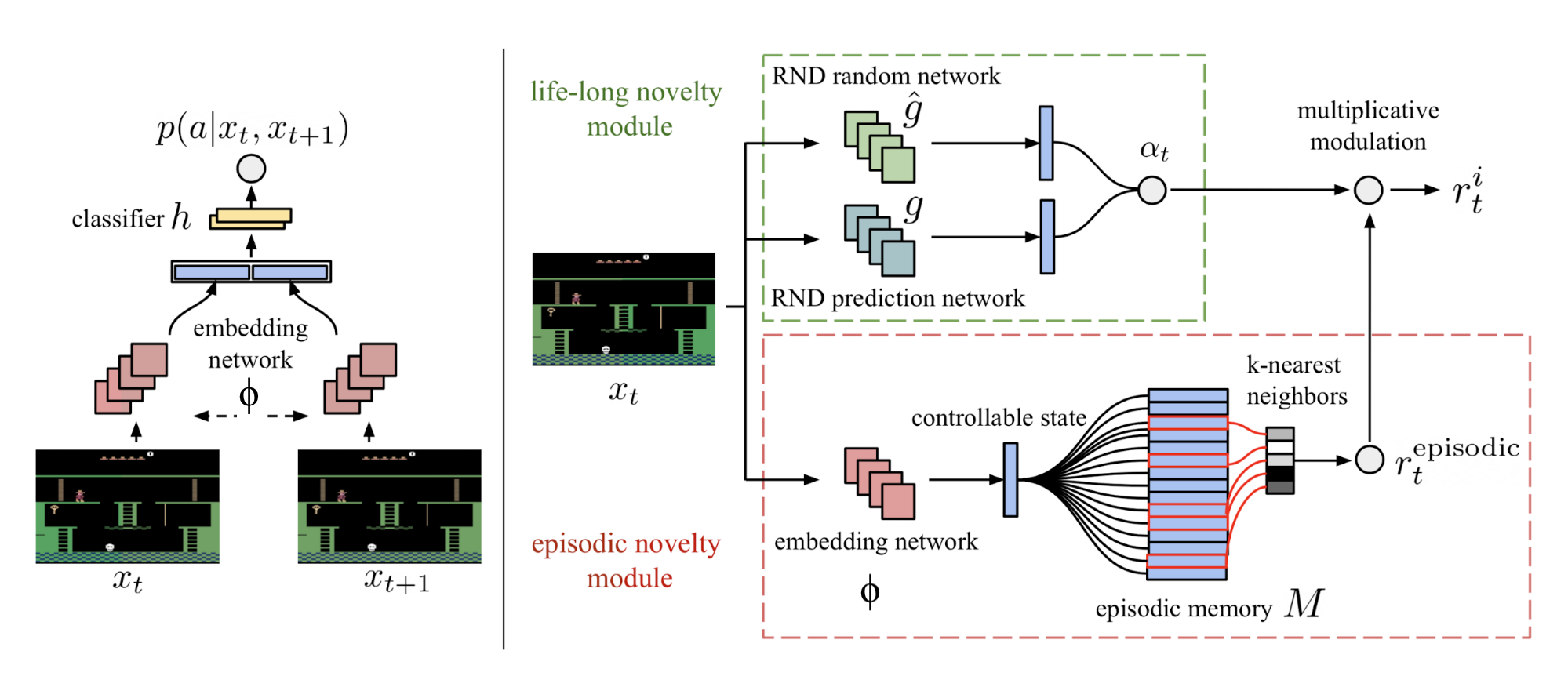
The long-term, across-episode novelty uses the RND prediction error as a life-long novelty module. The exploration bonus is $\alpha_t = 1 + \frac{e^\text{RND}(s_t) - \mu_e}{\sigma_e}$, where $\mu_e$ and $\sigma_e$ are the running mean and standard deviation for the RND error $e^\text{RND}(s_t)$.

However in the conclusion section of the RND paper, I noticed the following statement:

“We find that the RND exploration bonus is sufficient to deal with local exploration, i.e. exploring the consequences of short-term decisions, like whether to interact with a particular object, or avoid it. However global exploration that involves coordinated decisions over long time horizons is beyond the reach of our method. "

And this confuses me a bit how RND can be used as a good life-long novelty bonus provider. If you know why, feel free to leave a comment below.

The final intrinsic reward is the combined value $r^i_t = r^\text{episodic}_t \cdot \text{clip}(\alpha_t, 1, L)$, where $L$ is a constant maximum reward scalar.

This NGU design yields two desirable properties:

1. It rapidly discourages revisiting the same state within an episode.
2. It slowly discourages revisiting states that have been visited many times across episodes.

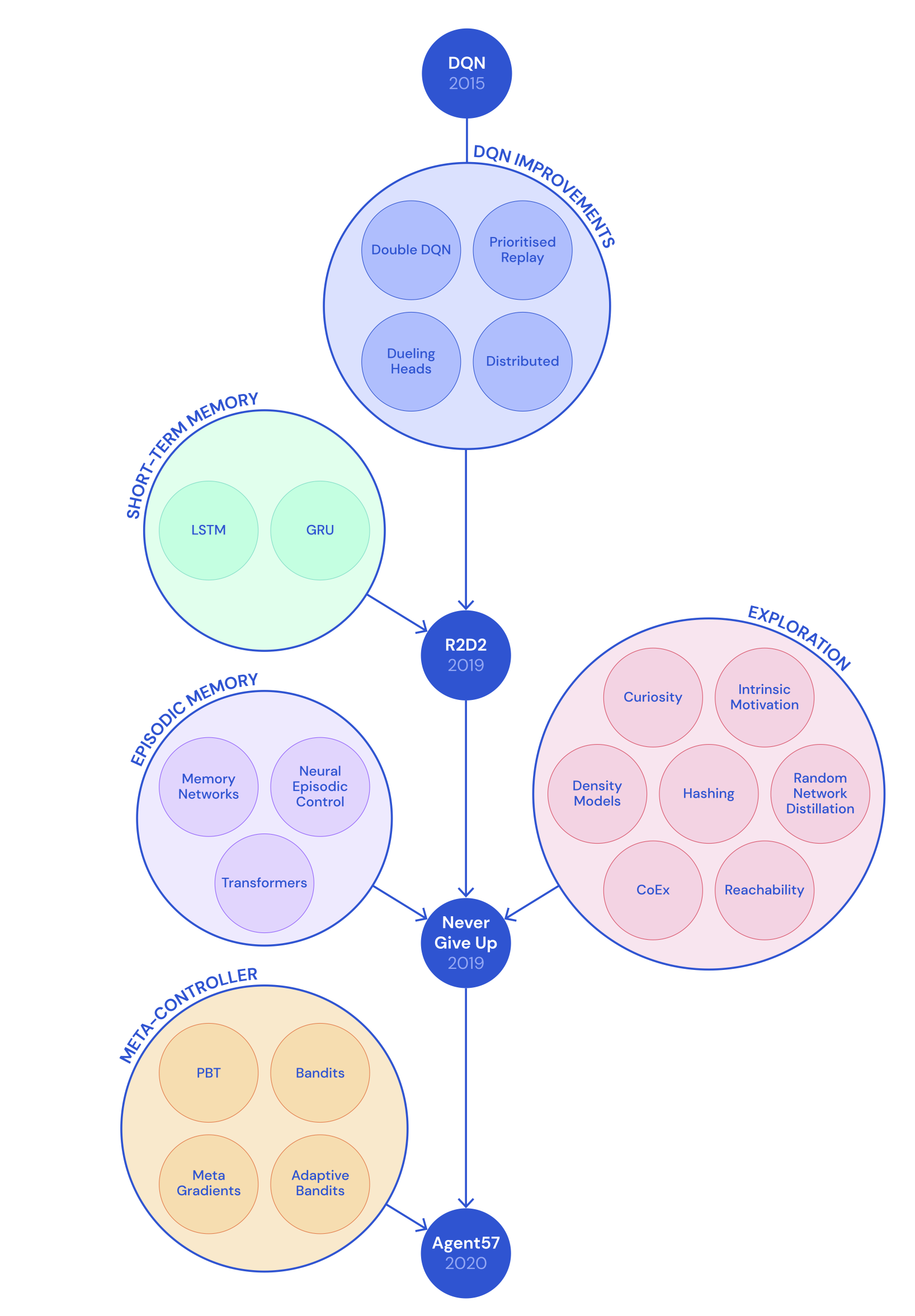
Building on NGU, DeepMind later introduced “Agent57” (Badia, et al. 2020b), the first deep RL agent to outperform the standard human benchmark on all 57 Atari games. Agent57 makes two primary improvements over NGU:

1. Agent57 trains a population of policies, each with a distinct exploration parameter pair $\{(\beta_j, \gamma_j)\}_{j=1}^N$. Recall that, given $\beta_j$, the reward is constructed as $r_{j,t} = r_t^e + \beta_j r^i_t$, and $\gamma_j$ is the reward discount factor. It is natural to expect that policies with higher $\beta_j$ and lower $\gamma_j$ will achieve more progress early in training, while the reverse may be expected later in training. A meta-controller (sliding-window UCB bandit algorithm) is trained to determine which policies should be prioritized.
2. The second improvement introduces a new Q-value parameterization that separates intrinsic and extrinsic reward contributions in a form similar to the bundled reward: $Q(s, a; \theta_j) = Q(s, a; \theta_j^e) + \beta_j Q(s, a; \theta_j^i)$. During training, $Q(s, a; \theta_j^e)$ and $Q(s, a; \theta_j^i)$ are optimized separately using rewards $r_j^e$ and $r_j^i$, respectively.

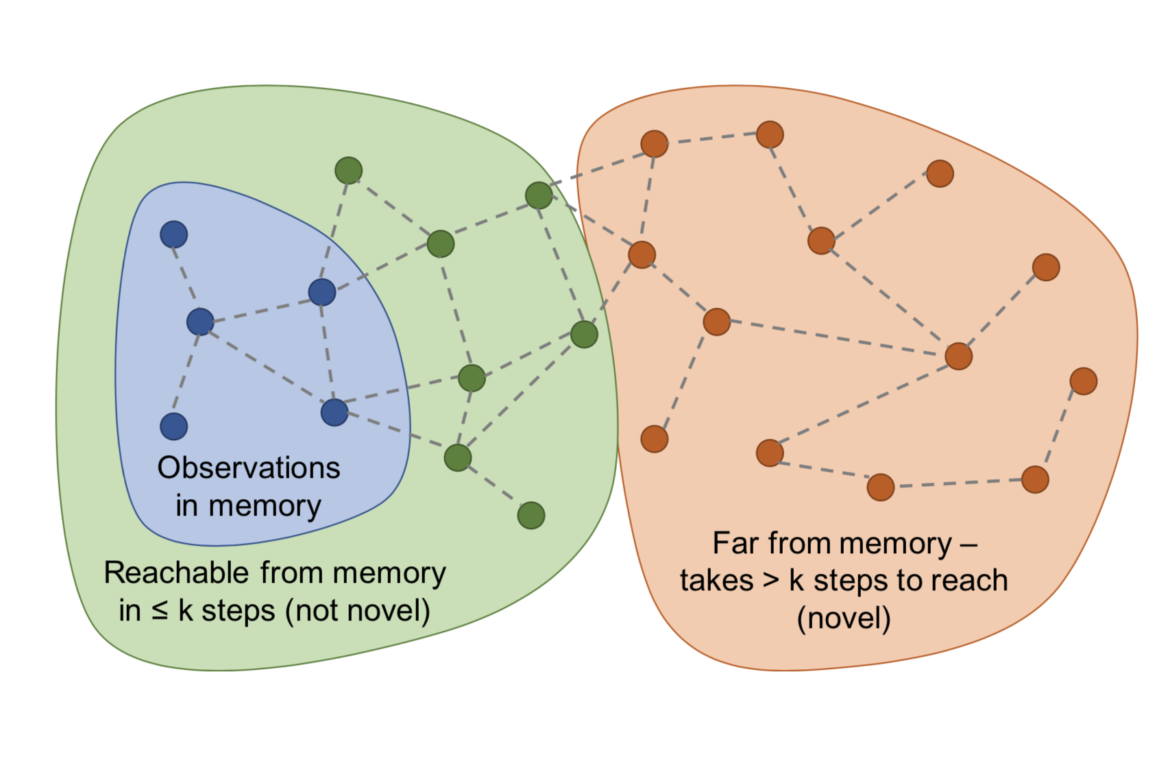
Rather than using Euclidean distance to measure state similarity in episodic memory, Savinov, et al. (2019) incorporated state-to-state transitions and proposed a method that estimates how many steps are required to reach one state from other states in memory. This method is called the Episodic Curiosity (EC) module, and its novelty bonus depends on state reachability.

1. At the start of each episode, the agent initializes an empty episodic memory $M$.
2. At each step, the agent compares the current state against stored states in memory to compute the novelty bonus: if the current state is novel (that is, it requires more steps to reach from memory observations than a threshold), the agent receives a bonus.
3. The current state is added to episodic memory if the novelty bonus is sufficiently large. (Intuitively, if all states were stored in memory, then any new state could be reached within 1 step.)
4. Steps 1 to 3 are repeated until the episode ends.

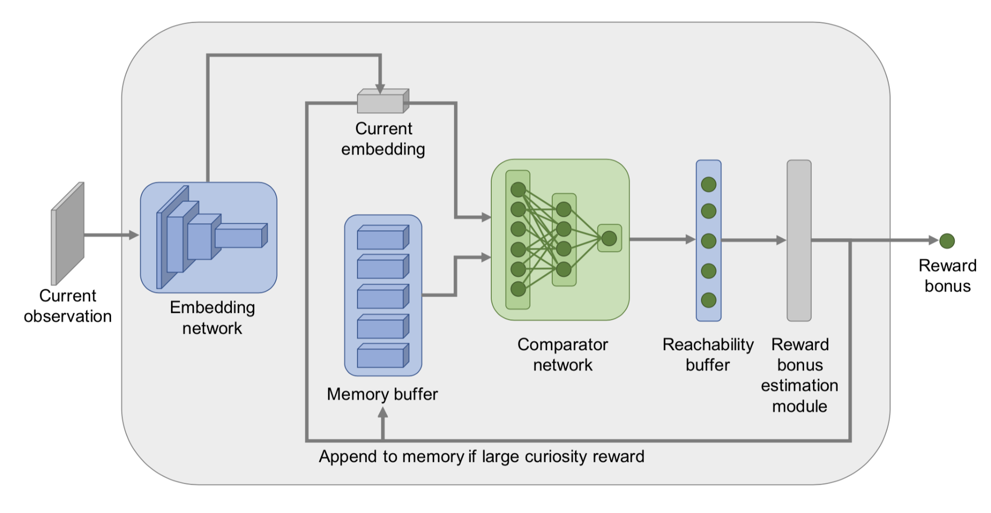
To estimate reachability between states, access to the transition graph is needed, but the graph is not fully known. Therefore, Savinov, et al. (2019) trained a siamese neural network to predict how many steps separate two states. The approach uses an embedding network $\phi: \mathcal{S} \mapsto \mathbb{R}^n$ to encode states as feature vectors, followed by a comparator network $C: \mathbb{R}^n \times \mathbb{R}^n \mapsto [0, 1]$ that outputs a binary label indicating whether two states are sufficiently close (that is, reachable within $k$ steps) in the transition graph, $C(\phi(s_i), \phi(s_j)) \mapsto [0, 1]$.

An episodic memory buffer $M$ stores embeddings from earlier observations within the same episode. Each new observation is compared against stored embeddings using $C$, and the resulting scores are aggregated (for example, max or 90th percentile) to produce a reachability score $C^M(\phi(s_t))$. The exploration bonus is $r^i_t = \big(C’ - C^M(f(s_t))\big)$, where $C’$ is a predefined threshold that determines the sign of the reward (for example, $C’=0.5$ works well for fixed-duration episodes). A high bonus is assigned to new states when they are not easily reachable from the states contained in the memory buffer.

They claimed that the EC module can overcome the noisy-TV problem.

Direct Exploration

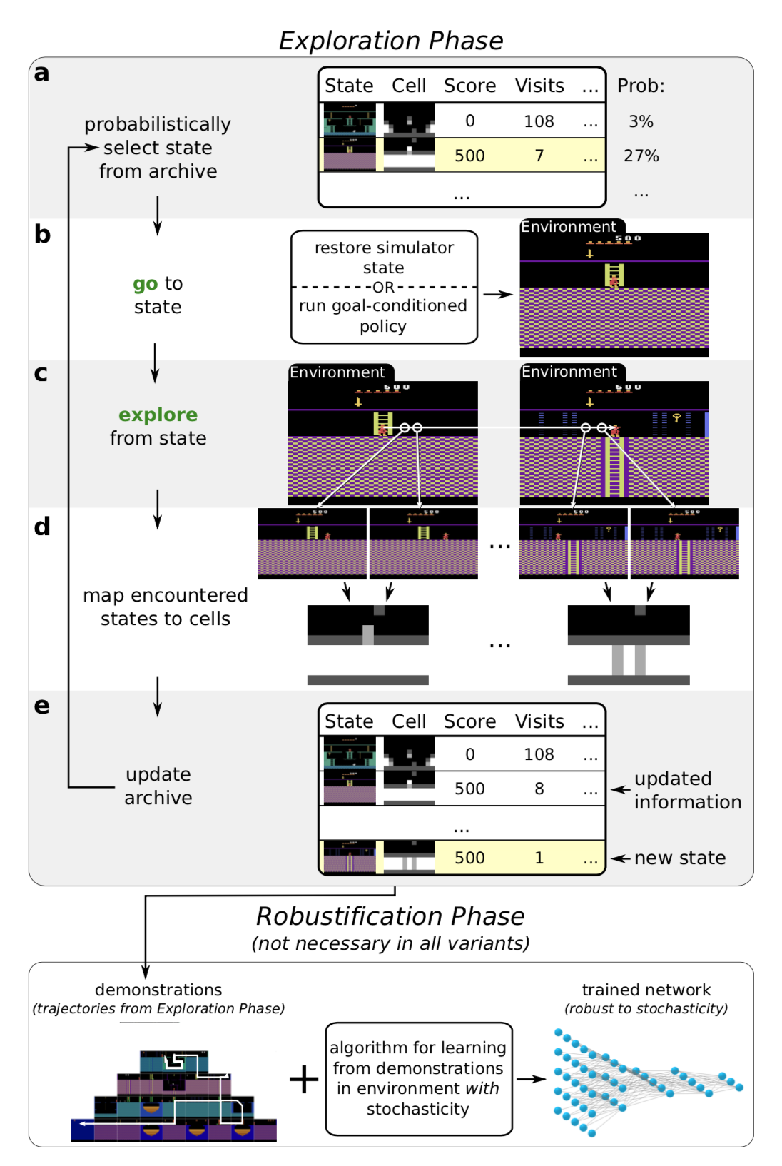
Go-Explore (Ecoffet, et al., 2019) is an algorithm designed to address the “hard-exploration” problem. It consists of two phases.

Phase 1 (“Explore until solved”) is conceptually similar to Dijkstra’s algorithm for finding shortest paths in a graph. In Phase 1, no neural networks are used. By maintaining a memory of interesting states and the trajectories that reach them, the agent can return (assuming a deterministic simulator) to promising states and continue random exploration from those points. To support memorization, each state is mapped to a compact discretized code (a “cell”). The memory is updated whenever a new state is discovered or when a better or shorter trajectory to a known state is found. When selecting a past state to revisit, the agent may sample uniformly from memory or follow heuristics such as recency, visit count, or the number of neighboring cells in memory. This process continues until the task is solved and at least one solution trajectory has been identified.

The high-performance trajectories found in Phase 1 do not transfer well to evaluation environments with stochasticity. As a result, Phase 2 (“Robustification”) is used to make the solution robust through imitation learning. The method adopts Backward Algorithm, where the agent is initialized near the final state of the trajectory and then performs RL optimization from that point.

An important caveat for Phase 1 is the following: to return deterministically to a prior state without exploration, Go-Explore requires a resettable and deterministic simulator, which is a substantial limitation.

To broaden applicability to stochastic environments, a later enhanced variant of Go-Explore (Ecoffet, et al., 2020), called policy-based Go-Explore, was introduced.

• Rather than resetting the simulator state directly, policy-based Go-Explore learns a goal-conditioned policy and uses it to repeatedly reach a known state stored in memory. The goal-conditioned policy is trained to follow the best trajectory that previously reached the selected memory states. A Self-Imitation Learning (SIL; Oh, et al. 2018) loss is included to extract as much information as possible from successful trajectories.
• They also report that sampling actions from a policy performs better than taking random actions when returning to promising states to continue exploration.
• A further improvement is an adjustable image downscaling function that maps images to cells. This function is optimized to avoid producing either too many or too few cells in memory.

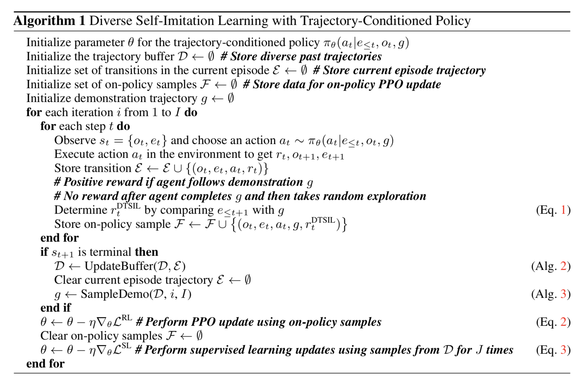
After vanilla Go-Explore, Yijie Guo, et al. (2019) proposed DTSIL (Diverse Trajectory-conditioned Self-Imitation Learning), which follows a similar overall approach to policy-based Go-Explore. DTSIL maintains a memory of diverse demonstrations collected during training and uses them to train a trajectory-conditioned policy via SIL. During sampling, it prioritizes trajectories that terminate in a rare state.

A related approach also appears in Guo, et al. (2019). The central idea is to store goals with high uncertainty in memory, enabling the agent to revisit these goal states repeatedly using a goal-conditioned policy. In each episode, the agent flips a coin (probability 0.5) to decide whether to act greedily with respect to the policy or to perform directed exploration by sampling goals from memory.

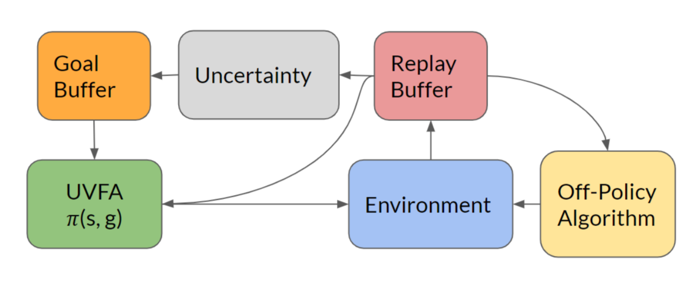
The uncertainty measure for a state can be simple (for example, count-based bonuses) or more complex (for example, density models or Bayesian models). The paper trains a forward dynamics model and uses its prediction error as the uncertainty metric.

Q-Value Exploration

Inspired by Thompson sampling, Bootstrapped DQN (Osband, et al. 2016) introduces uncertainty into Q-value approximation in classic DQN using the bootstrapping method. Bootstrapping approximates a distribution by repeatedly sampling, with replacement, from the same population and aggregating the results.

Multiple Q-value heads are trained in parallel. However, each head trains only on a bootstrapped subsample of the data and maintains its own target network. All Q-value heads share the same backbone network.

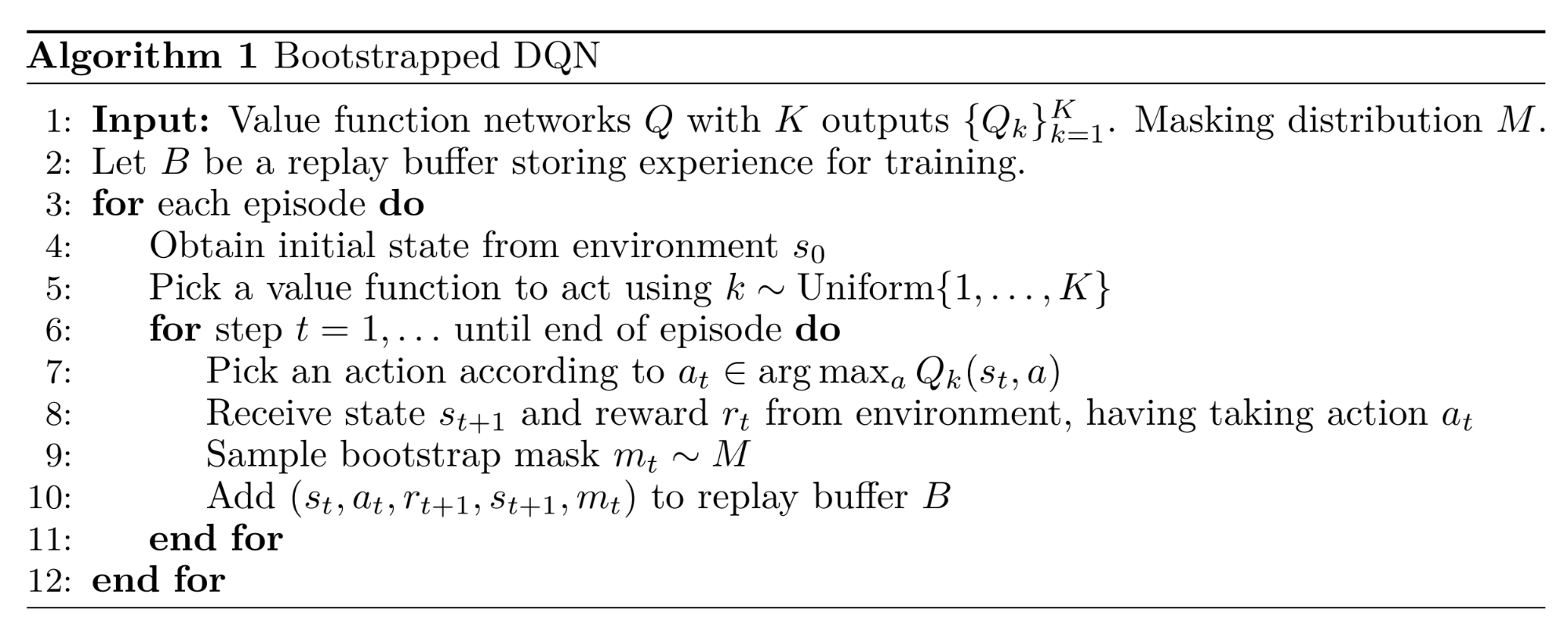
At the start of each episode, one Q-value head is sampled uniformly and is used for action selection while collecting experience during that episode. A binary mask is then sampled from the masking distribution $m \sim \mathcal{M}$ to determine which heads may use that data for training. The choice of masking distribution $\mathcal{M}$ determines how bootstrapped samples are formed. For example:

• If $\mathcal{M}$ is an independent Bernoulli distribution with $p=0.5$, this corresponds to the double-or-nothing bootstrap.
• If $\mathcal{M}$ always returns an all-one mask, the algorithm reduces to an ensemble method.

Despite this, the exploration remains limited because the uncertainty introduced through bootstrapping depends entirely on the training data. It is preferable to inject prior information that is independent of the data. This “noisy” prior is intended to keep the agent exploring under sparse rewards. The method of adding a random prior to bootstrapped DQN to improve exploration (Osband, et al. 2018) is based on Bayesian linear regression. The key idea in Bayesian regression is that we can “generate posterior samples by training on noisy versions of the data, together with some random regularization”.

Let $\theta$ denote the Q-function parameters and $\theta^-$ the target Q. The loss function with a randomized prior function $p$ is:

Varitional Options

Options are policies with termination conditions. The option search space contains many options, and these options are independent of the agent’s intentions. By explicitly modeling intrinsic options, an agent can receive intrinsic rewards that support exploration.

VIC (short for “Variational Intrinsic Control”; Gregor, et al. 2017) is a framework that provides intrinsic exploration bonuses by modeling options and learning option-conditioned policies. Let $\Omega$ denote an option that starts from $s_0$ and ends at $s_f$. An environment probability distribution $p^J(s_f \vert s_0, \Omega)$ specifies where an option $\Omega$ terminates given a starting state $s_0$. A controllability distribution $p^C(\Omega \vert s_0)$ specifies the distribution over options from which we can sample. By definition, $p(s_f, \Omega \vert s_0) = p^J(s_f \vert s_0, \Omega) p^C(\Omega \vert s_0)$ holds.

When selecting options, we aim to satisfy two objectives:

• Produce a diverse set of terminal states from $s_0$, which corresponds to maximizing $H(s_f \vert s_0)$.
• Determine precisely which final state a given option $\Omega$ will reach, which corresponds to minimizing $H(s_f \vert s_0, \Omega)$.

Combining these objectives yields the mutual information term $I(\Omega; s_f \vert s_0)$ to maximize:

Since mutual information is symmetric, we can interchange $s_f$ and $\Omega$ at multiple points without affecting the equivalence. In addition, because $p(\Omega \vert s_0, s_f)$ is hard to observe directly, we replace it with an approximate distribution, $q$. By the variational lower bound, this yields $I(\Omega; s_f \vert s_0) \geq I^{VB}(\Omega; s_f \vert s_0)$.

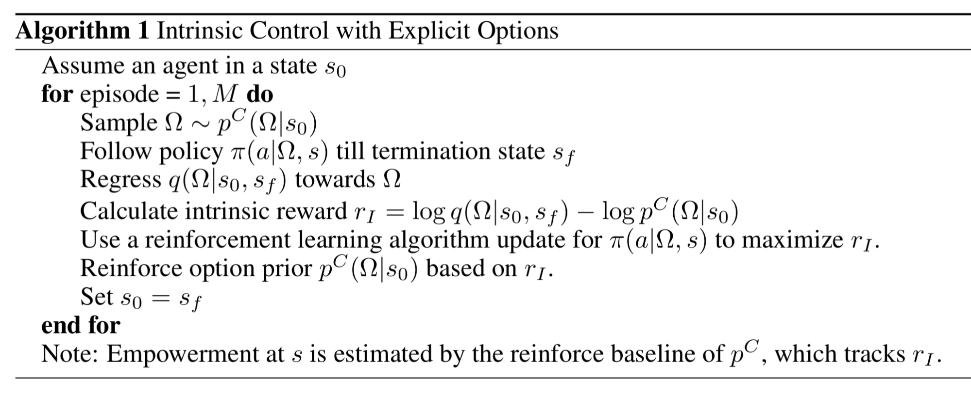
In this setup, $\pi(a \vert \Omega, s)$ can be optimized using any reinforcement learning algorithm. The option inference function, $q(\Omega \vert s_0, s_f)$, is trained via supervised learning. The prior, $p^C$, is updated so that it increasingly selects $\Omega$ that produce higher rewards. Note that $p^C$ may also be held fixed (for example, as a Gaussian). Different choices of $\Omega$ lead to different learned behaviors. Furthermore, Gregor, et al. (2017) noted that, in practice, it is difficult to make VIC with explicit options work well under function approximation, and they therefore proposed an alternative variant of VIC based on implicit options.

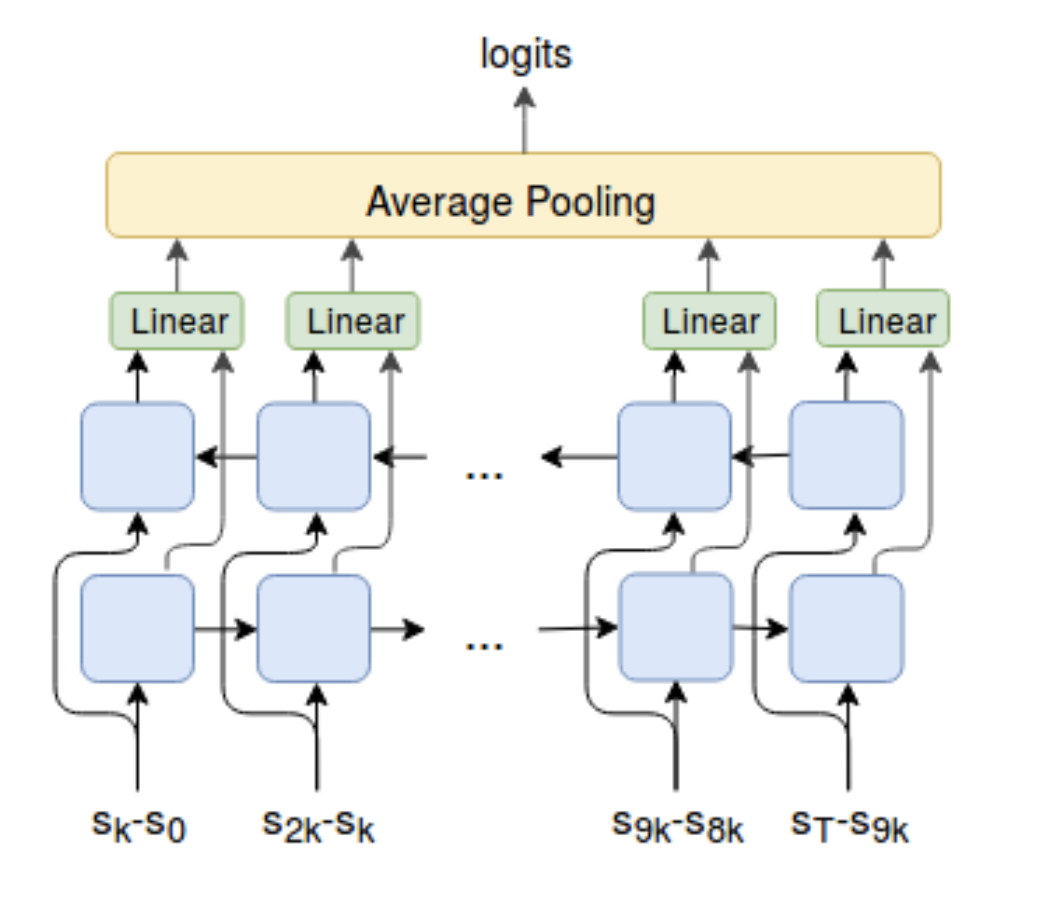
Unlike VIC, which models $\Omega$ conditioned only on the start and end states, VALOR (short for “Variational Auto-encoding Learning of Options by Reinforcement”; Achiam, et al. 2018) uses the full trajectory to extract the option context $c$, sampled from a fixed Gaussian distribution. In VALOR:

• A policy serves as an encoder, mapping contexts drawn from a noise distribution to trajectories.
• A decoder attempts to reconstruct the contexts from the trajectories and provides rewards to policies that make contexts easier to distinguish. During training, the decoder never observes the actions, so the agent must interact with the environment in a manner that supports effective communication with the decoder to improve prediction. The decoder also processes the sequence of steps in a trajectory recurrently to better capture correlations across timesteps.

DIAYN (“Diversity is all you need”; Eysenbach, et al. 2018) follows the same general direction, although it uses different terminology: DIAYN models policies conditioned on a latent skill variable. See my previous post for additional details.

Citation

Cited as:

Weng, Lilian. (Jun 2020). Exploration strategies in deep reinforcement learning. Lil’Log. https://lilianweng.github.io/posts/2020-06-07-exploration-drl/.

Or

@article{weng2020exploration,
  title   = "Exploration Strategies in Deep Reinforcement Learning",
  author  = "Weng, Lilian",
  journal = "lilianweng.github.io",
  year    = "2020",
  month   = "Jun",
  url     = "https://lilianweng.github.io/posts/2020-06-07-exploration-drl/"
}

Reference

[1] Pierre-Yves Oudeyer & Frederic Kaplan. “How can we define intrinsic motivation?” Conf. on Epigenetic Robotics, 2008.

[2] Marc G. Bellemare, et al. “Unifying Count-Based Exploration and Intrinsic Motivation”. NIPS 2016.

[3] Georg Ostrovski, et al. “Count-Based Exploration with Neural Density Models”. PMLR 2017.

[4] Rui Zhao & Volker Tresp. “Curiosity-Driven Experience Prioritization via Density Estimation”. NIPS 2018.

[5] Haoran Tang, et al. "#Exploration: A Study of Count-Based Exploration for Deep Reinforcement Learning”. NIPS 2017.

[6] Jürgen Schmidhuber. “A possibility for implementing curiosity and boredom in model-building neural controllers” 1991.

[7] Pierre-Yves Oudeyer, et al. “Intrinsic Motivation Systems for Autonomous Mental Development” IEEE Transactions on Evolutionary Computation, 2007.

[8] Bradly C. Stadie, et al. “Incentivizing Exploration In Reinforcement Learning With Deep Predictive Models”. ICLR 2016.

[9] Deepak Pathak, et al. “Curiosity-driven Exploration by Self-supervised Prediction”. CVPR 2017.

[10] Yuri Burda, Harri Edwards & Deepak Pathak, et al. “Large-Scale Study of Curiosity-Driven Learning”. arXiv 1808.04355 (2018).

[11] Joshua Achiam & Shankar Sastry. “Surprise-Based Intrinsic Motivation for Deep Reinforcement Learning” NIPS 2016 Deep RL Workshop.

[12] Rein Houthooft, et al. “VIME: Variational information maximizing exploration”. NIPS 2016.

[13] Leshem Choshen, Lior Fox & Yonatan Loewenstein. “DORA the explorer: Directed outreaching reinforcement action-selection”. ICLR 2018

[14] Yuri Burda, et al. “Exploration by Random Network Distillation” ICLR 2019.

[15] OpenAI Blog: “Reinforcement Learning with Prediction-Based Rewards” Oct, 2018.

[16] Misha Denil, et al. “Learning to Perform Physics Experiments via Deep Reinforcement Learning”. ICLR 2017.

[17] Ian Osband, et al. “Deep Exploration via Bootstrapped DQN”. NIPS 2016.

[18] Ian Osband, John Aslanides & Albin Cassirer. “Randomized Prior Functions for Deep Reinforcement Learning”. NIPS 2018.

[19] Karol Gregor, Danilo Jimenez Rezende & Daan Wierstra. “Variational Intrinsic Control”. ICLR 2017.

[20] Joshua Achiam, et al. “Variational Option Discovery Algorithms”. arXiv 1807.10299 (2018).

[21] Benjamin Eysenbach, et al. “Diversity is all you need: Learning skills without a reward function.”. ICLR 2019.

[22] Adrià Puigdomènech Badia, et al. “Never Give Up (NGU): Learning Directed Exploration Strategies” ICLR 2020.

[23] Adrià Puigdomènech Badia, et al. “Agent57: Outperforming the Atari Human Benchmark”. arXiv 2003.13350 (2020).

[24] DeepMind Blog: “Agent57: Outperforming the human Atari benchmark” Mar 2020.

[25] Nikolay Savinov, et al. “Episodic Curiosity through Reachability” ICLR 2019.

[26] Adrien Ecoffet, et al. “Go-Explore: a New Approach for Hard-Exploration Problems”. arXiv 1901.10995 (2019).

[27] Adrien Ecoffet, et al. “First return then explore”. arXiv 2004.12919 (2020).

[28] Junhyuk Oh, et al. “Self-Imitation Learning”. ICML 2018.

[29] Yijie Guo, et al. “Self-Imitation Learning via Trajectory-Conditioned Policy for Hard-Exploration Tasks”. arXiv 1907.10247 (2019).

[30] Zhaohan Daniel Guo & Emma Brunskill. “Directed Exploration for Reinforcement Learning”. arXiv 1906.07805 (2019).

[31] Deepak Pathak, et al. “Self-Supervised Exploration via Disagreement.” ICML 2019.