Learning with Insufficient Data, Part 2: Active Learning
This is Part 2 of our discussion on how to proceed when you have only a limited amount of labeled data for supervised learning tasks. In this installment, we introduce a controlled amount of human labeling effort, constrained by a fixed budget. Accordingly, we must be deliberate and efficient in deciding which samples to send for labeling.
· 22 min read · Curated and presented by Arthur Sedek
Supervised learning performance generally improves as more high-quality labels become available. However, collecting large labeled datasets is expensive. Active learning is a practical paradigm for situations with insufficient labeled data, where additional labeling is possible but must fit within a limited budget.
This is part 2 of a series on what to do when you have only a limited amount of labeled data for supervised learning tasks. Here, we incorporate a certain amount of human labeling effort, constrained by a budget, so we must be strategic about which samples to label.
Notations
| Symbol | Meaning |
|---|---|
| $K$ | Number of unique class labels. |
| $(\mathbf{x}^l, y) \sim \mathcal{X}, y \in \{0, 1\}^K$ | Labeled dataset. $y$ is a one-hot representation of the true label. |
| $\mathbf{u} \sim \mathcal{U}$ | Unlabeled dataset. |
| $\mathcal{D} = \mathcal{X} \cup \mathcal{U}$ | The entire dataset, including both labeled and unlabeled examples. |
| $\mathbf{x}$ | Any sample which can be either labeled or unlabeled. |
| $\mathbf{x}_i$ | The $i$-th sample. |
| $U(\mathbf{x})$ | Scoring function for active learning selection. |
| $P_\theta(y \vert \mathbf{x})$ | A softmax classifier parameterized by $\theta$. |
| $\hat{y} = \arg\max_{y \in \mathcal{Y}} P_\theta(y \vert \mathbf{x})$ | The most confident prediction by the classifier. |
| $B$ | Labeling budget (the maximum number of samples to label). |
| $b$ | Batch size. |
What is Active Learning?
Given an unlabeled dataset $\mathcal{U}$ and a fixed labeling budget $B$, active learning aims to choose a subset of $B$ examples from $\mathcal{U}$ for labeling such that model performance improves as much as possible. This approach is particularly effective when labeling is difficult and costly (for example, for medical images). The classical survey paper from 2010 summarizes many core concepts. Although some conventional approaches may not transfer directly to deep learning, this post focuses primarily on deep neural models trained in batch mode.
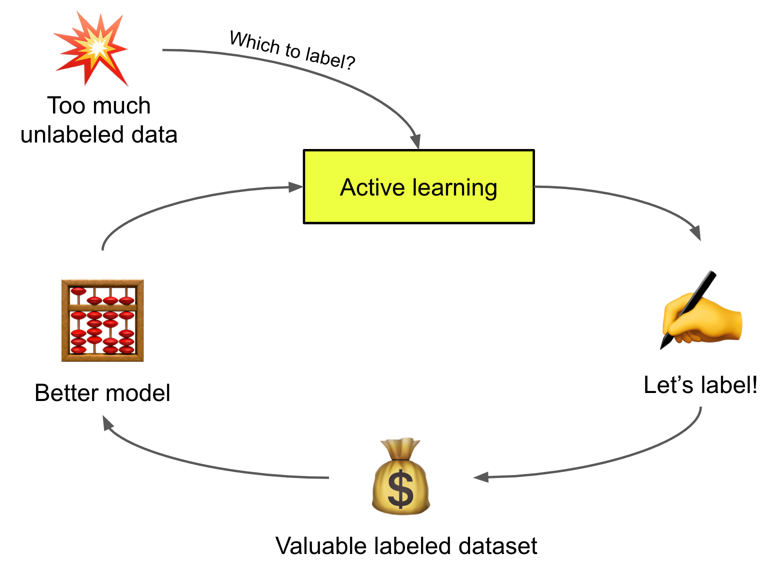
To streamline the discussion, we assume throughout that the task is a $K$-class classification problem. A model with parameters $\theta$ produces a probability distribution over candidate labels (which may or may not be calibrated), $P_\theta(y \vert \mathbf{x})$, and its most likely prediction is $\hat{y} = \arg\max_{y \in \mathcal{Y}} P_\theta(y \vert \mathbf{x})$.
Acquisition Function
The process of determining which examples are most valuable to label next is commonly called a “sampling strategy” or “query strategy”. The scoring function used during sampling is referred to as the “acquisition function”, denoted $U(\mathbf{x})$. Data points that receive higher scores are expected to provide more benefit to model training once labeled.
Below are several fundamental sampling strategies.
Uncertainty Sampling
Uncertainty sampling prioritizes examples for which the model is most uncertain. For a single model, uncertainty is often estimated from predicted probabilities. A frequent criticism, however, is that deep learning predictions are often poorly calibrated and may not reflect true uncertainty well. Indeed, deep models are often overconfident.
- Least confident score, also called the variation ratio: $U(\mathbf{x}) = 1 - P_\theta(\hat{y} \vert \mathbf{x})$.
- Margin score: $U(\mathbf{x}) = P_\theta(\hat{y}_1 \vert \mathbf{x}) - P_\theta(\hat{y}_2 \vert \mathbf{x})$, where $\hat{y}_1$ and $\hat{y}_2$ are the most likely and second most likely predicted labels.
- Entropy: $U(\mathbf{x}) = \mathcal{H}(P_\theta(y \vert \mathbf{x})) = - \sum_{y \in \mathcal{Y}} P_\theta(y \vert \mathbf{x}) \log P_\theta(y \vert \mathbf{x})$.
Uncertainty can also be quantified using a committee of expert models, known as Query-By-Committee (QBC). QBC estimates uncertainty by aggregating multiple opinions, so it is important to maintain meaningful disagreement across committee members. Suppose the committee contains $C$ models, each parameterized by $\theta_1, \dots, \theta_C$.
- Voter entropy: $U(\mathbf{x}) = \mathcal{H}(\frac{V(y)}{C})$, where $V(y)$ counts how many committee members vote for label $y$.
- Consensus entropy: $U(\mathbf{x}) = \mathcal{H}(P_\mathcal{C})$, where $P_\mathcal{C}$ is the committee-averaged prediction.
- KL divergence: $U(\mathbf{x}) = \frac{1}{C} \sum_{c=1}^C D_\text{KL} (P_{\theta_c} | P_\mathcal{C})$
Diversity Sampling
Diversity sampling aims to identify a set of samples that represents the overall data distribution well. Diversity matters because the model is expected to perform reliably on real-world data, rather than only on a narrow subset. Accordingly, selected samples should be representative of the underlying distribution. Many common methods rely on measuring similarity between samples.
Expected Model Change
Expected model change captures how much a sample is expected to influence training. This influence may be expressed as a change in model weights or as an improvement in the training loss. A later section reviews several works that measure training impact attributable to selected samples.
Hybrid Strategy
The methods above are not mutually exclusive. A hybrid strategy assigns value to multiple attributes of a data point, combining different sampling preferences into a single approach. In many settings, we want to select uncertain but also highly representative samples.
Deep Acquisition Function
Measuring Uncertainty
Model uncertainty is commonly grouped into two categories (Der Kiureghian & Ditlevsen 2009, Kendall & Gal 2017):
- Aleatoric uncertainty arises from noise in the data (for example, sensor noise or measurement noise). It may be input-dependent or input-independent. It is generally viewed as irreducible because information about the ground truth is missing.
- Epistemic uncertainty reflects uncertainty in model parameters, meaning we are unsure whether the model best explains the data. This uncertainty is theoretically reducible with more data.
Ensemble and Approximated Ensemble
Machine learning has a long history of using ensembles to improve performance. When models are sufficiently diverse, ensembles are expected to deliver better results. This principle is validated across many ML algorithms. For example, AdaBoost combines many weak learners to match, or sometimes outperform, a single strong learner. Bootstrapping ensembles repeated resampling trials to produce more accurate metric estimates. Random forests and GBM are also well-known demonstrations of effective ensembling.
For improved uncertainty estimation, it is natural to aggregate multiple independently trained models. However, training even one deep neural network can be expensive, and training many is often impractical. In reinforcement learning, Bootstrapped DQN (Osband, et al. 2016) uses multiple value heads and leverages uncertainty across an ensemble of Q-value approximations to guide exploration in RL.
In active learning, a more common approach is to use dropout to “simulate” a probabilistic Gaussian process (Gal & Ghahramani 2016). The idea is to ensemble multiple stochastic forward passes from a single model, each using a different dropout mask, to estimate model (epistemic) uncertainty. This is referred to as MC dropout (Monte Carlo dropout). When dropout is applied before every weight layer, it is shown to be mathematically equivalent to an approximation of a probabilistic deep Gaussian process (Gal & Ghahramani 2016). This simple technique has proven effective for small-data classification and is widely used when efficient uncertainty estimation is needed.
DBAL (Deep Bayesian active learning; Gal et al. 2017) approximates Bayesian neural networks using MC dropout, enabling learning a distribution over model weights. In their experiments, MC dropout outperformed a random baseline and mean standard deviation (Mean STD), and performed similarly to variation ratios and entropy-based measures.
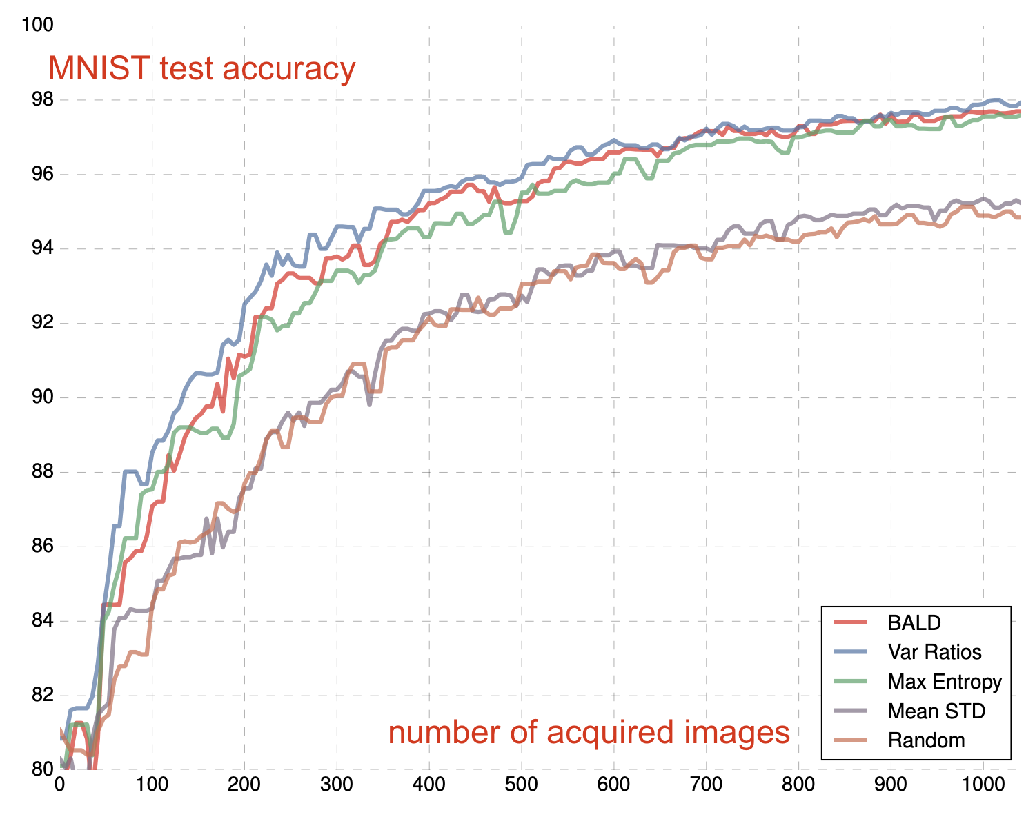
Beluch et al. (2018) compared ensemble-based models against MC dropout and found that combining a naive ensemble (training multiple models separately and independently) with the variation ratio provides better-calibrated predictions than other approaches. However, naive ensembles are very expensive, so they explored several cheaper alternatives:
- Snapshot ensemble: Train an implicit ensemble using a cyclic learning rate schedule so that optimization converges to different local minima.
- Diversity encouraging ensemble (DEE): Start from a base network trained for a small number of epochs, then use it to initialize $n$ different networks, each trained with dropout to encourage diversity.
- Split head approach: Use one base model with multiple heads, where each head corresponds to one classifier.
Unfortunately, all of the lower-cost implicit ensemble options above underperform naive ensembles. Given constraints on computational resources, MC dropout remains a strong and economical choice. It is also natural to combine ensembles with MC dropout (Pop & Fulop 2018) to gain additional performance via stochastic ensembling.
Uncertainty in Parameter Space
Bayes-by-backprop (Blundell et al. 2015) measures uncertainty in neural network weights directly. The method maintains a probability distribution over weights $\mathbf{w}$, represented as a variational distribution $q(\mathbf{w} \vert \theta)$ because the true posterior $p(\mathbf{w} \vert \mathcal{D})$ is not directly tractable. The objective minimizes the KL divergence between $q(\mathbf{w} \vert \theta)$ and $p(\mathbf{w} \vert \mathcal{D})$:
The variational distribution $q$ is typically a diagonal-covariance Gaussian, and each weight is sampled from $\mathcal{N}(\mu_i, \sigma_i^2)$. To ensure that $\sigma_i$ is non-negative, it is parameterized using softplus, $\sigma_i = \log(1 + \exp(\rho_i))$, where the variational parameters are $\theta = \{\mu_i , \rho_i\}^d_{i=1}$.
The Bayes-by-backprop procedure can be summarized as follows:
- Sample $\epsilon \sim \mathcal{N}(0, I)$
- Let $\mathbf{w} = \mu + \log(1+ \exp(\rho)) \circ \epsilon$
- Let $\theta = (\mu, \rho)$
- Let $f(\mathbf{w}, \theta) = \log q(\mathbf{w} \vert \theta) - \log p(\mathbf{w})p(\mathcal{D}\vert \mathbf{w})$
- Compute the gradient of $f(\mathbf{w}, \theta)$ with respect to $\mu$ and $\rho$, then update $\theta$.
- Measure uncertainty by sampling different model weights during inference.
Loss Prediction
The loss objective drives training, and low loss values indicate that the model is producing accurate predictions. Yoo & Kweon (2019) introduced a loss prediction module that predicts the loss value for unlabeled inputs, providing an estimate of how well the model is likely to perform on a given sample. Samples are selected when the loss prediction module produces uncertain outputs (high predicted loss). The module is a simple MLP with dropout. It consumes intermediate layer features, applies global average pooling, and concatenates the resulting vectors.
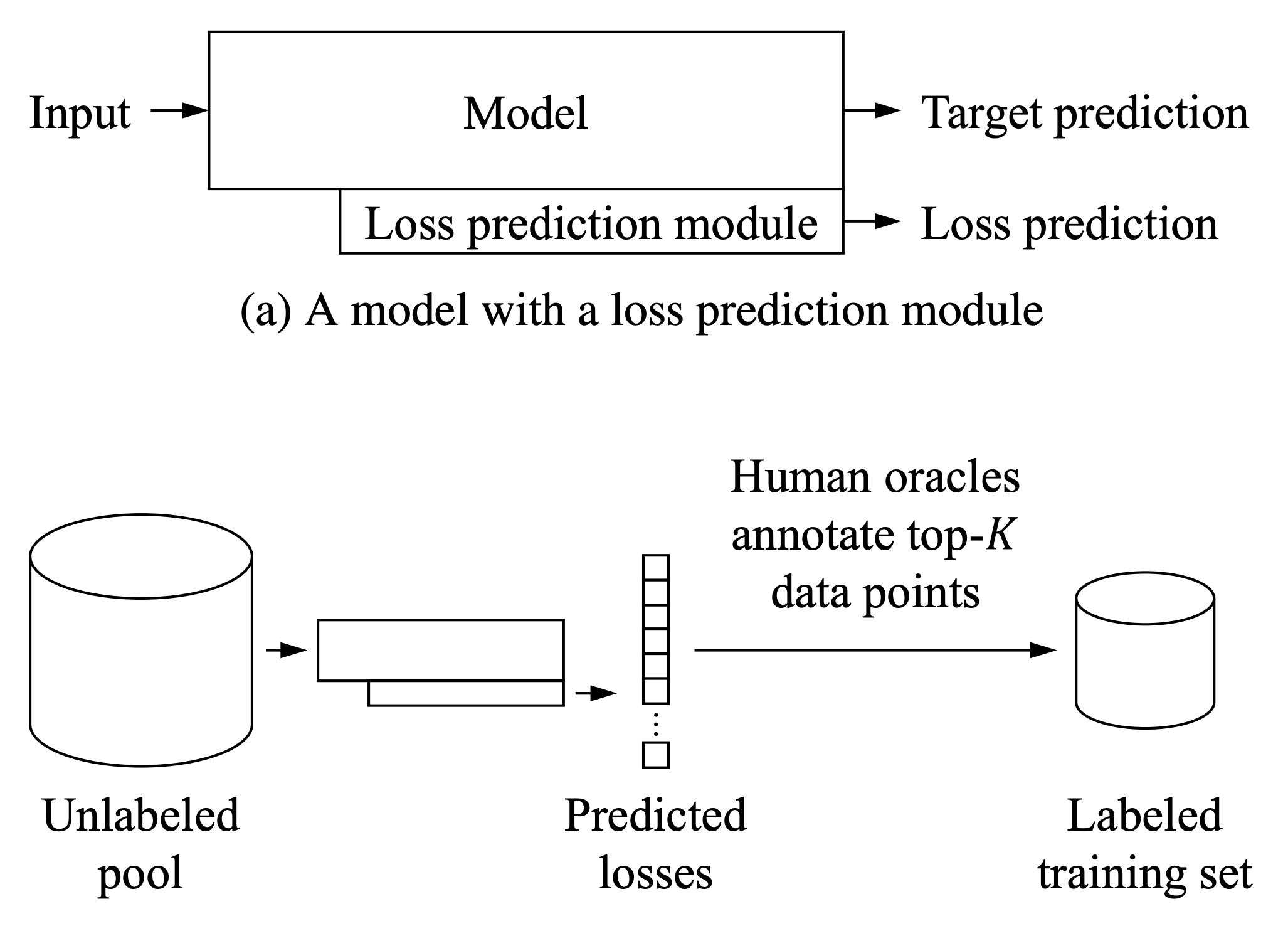
Let $\hat{l}$ denote the loss prediction module output and $l$ denote the true loss. When training the loss prediction module, a straightforward MSE loss $=(l - \hat{l})^2$ is not ideal because the loss decreases over time as the model improves. Therefore, an effective objective should not depend on changes in the target loss scale. Instead, they formulate training as a pairwise comparison task. For a batch of size $b$, there are $b/2$ sample pairs $(\mathbf{x}_i, \mathbf{x}_j)$, and the loss prediction model should correctly predict which sample in the pair has the larger loss.
where $\epsilon$ is a predefined positive margin constant.
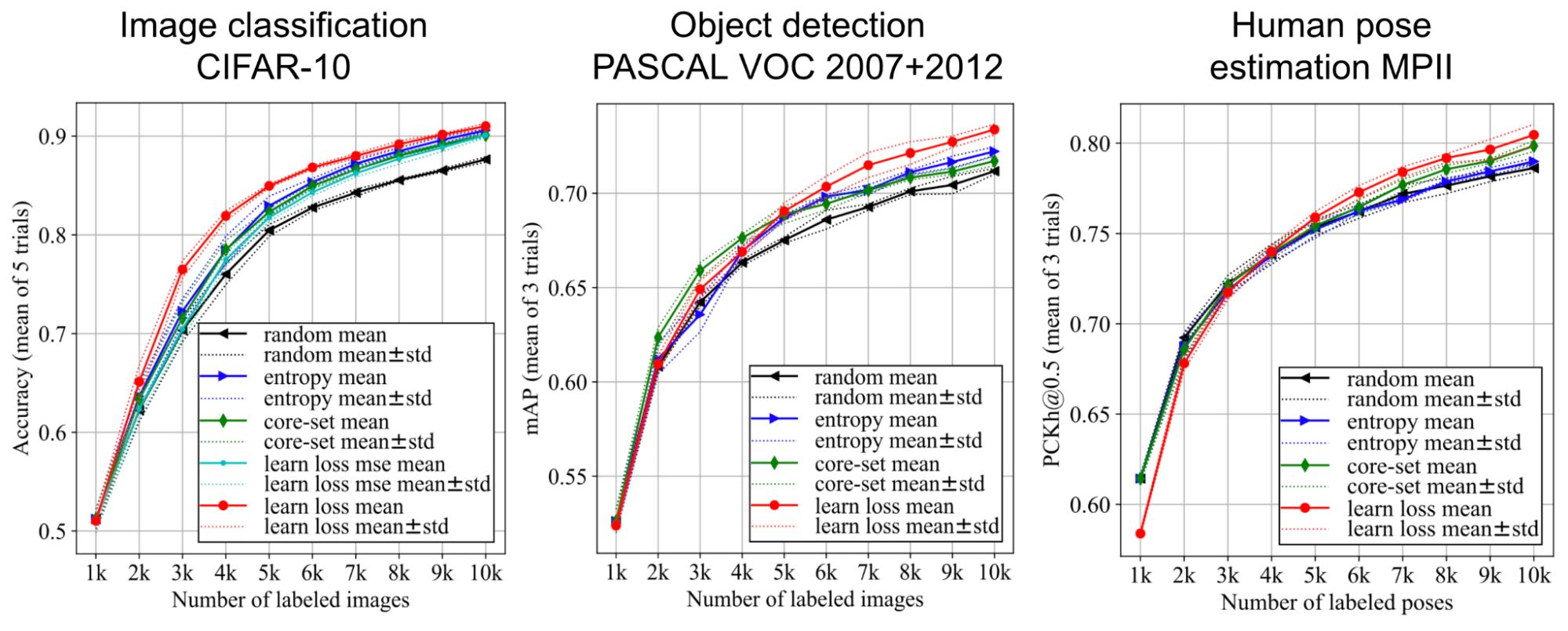
Across three vision tasks, active learning based on the loss prediction module outperformed a random baseline, entropy-based acquisition, and the core-set method.
Adversarial Setup
Sinha et al. (2019) proposed a GAN-like approach called VAAL (Variational Adversarial Active Learning). In VAAL, a discriminator is trained to distinguish unlabeled data from labeled data. Notably, in VAAL the acquisition criterion does not depend on task performance.
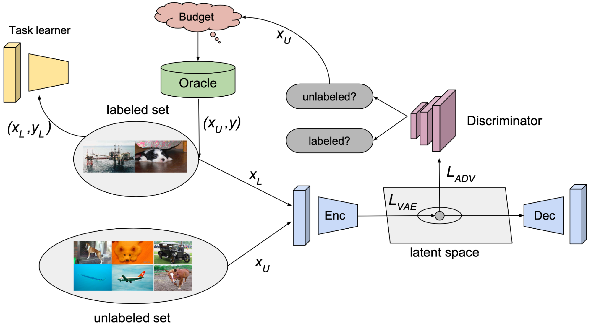
- The $\beta$-VAE learns a latent feature space $\mathbf{z}^l \cup \mathbf{z}^u$ for labeled and unlabeled data, respectively, with the goal of tricking the discriminator $D(.)$ into treating all data points as if they came from the labeled pool.
- The discriminator $D(.)$ predicts whether a sample is labeled (1) or unlabeled (0) based on latent representation $\mathbf{z}$. VAAL selects unlabeled samples with low discriminator scores, indicating that these samples differ sufficiently from previously labeled data.
The VAE representation-learning loss in VAAL includes both a reconstruction term (minimizing the ELBO for samples) and an adversarial term (labeled and unlabeled data are drawn from the same probability distribution $q_\phi$):
where $p(\mathbf{\tilde{z}})$ is a unit Gaussian prior and $\beta$ is the Lagrangian parameter.
The discriminator loss is:
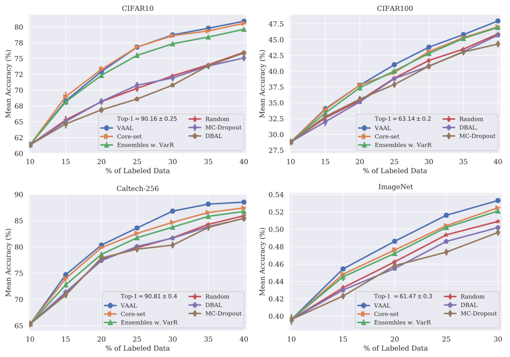
Ablation studies showed that jointly training the VAE and discriminator is essential. The results are robust to a biased initial labeled pool, to different labeling budgets, and to a noisy oracle.
MAL (Minimax Active Learning; Ebrahimiet al. 2021) extends VAAL. The MAL framework includes an entropy-minimizing feature encoder $F$ followed by an entropy-maximizing classifier $C$. This minimax formulation reduces the distribution gap between labeled and unlabeled data.
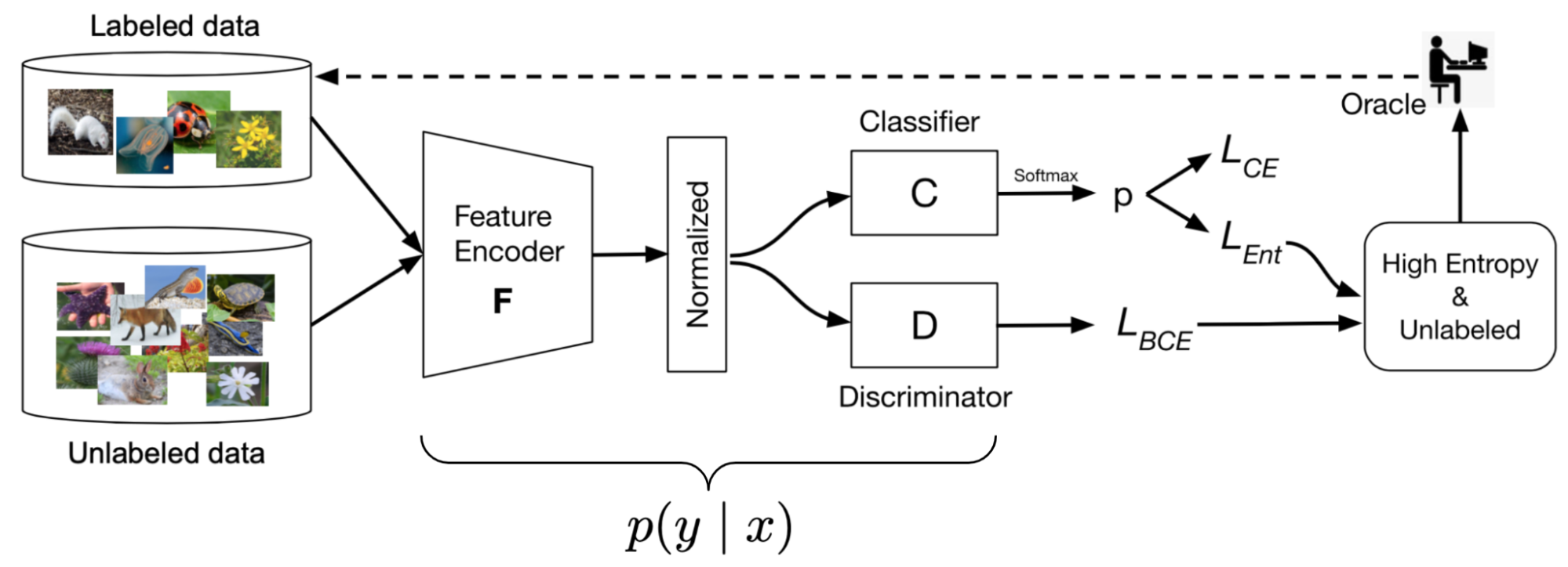
A feature encoder $F$ maps a sample to a $\ell_2$-normalized, $d$-dimensional latent vector. Assuming $K$ classes, a classifier $C$ is parameterized by $\mathbf{W} \in \mathbb{R}^{d \times K}$.
(1) First, $F$ and $C$ are trained on labeled samples using standard cross-entropy to achieve strong classification performance:
(2) For unlabeled examples, MAL adopts a minimax game:
where:
- Minimizing the entropy in $F$ encourages unlabeled samples with similar predicted labels to have similar features.
- Maximizing the entropy in $C$ adversarially pushes predictions toward a more uniform class distribution. (My understanding here is that because the true label of an unlabeled sample is unknown, we should not optimize the classifier to maximize the predicted labels just yet.)
The discriminator is trained in the same manner as in VAAL.
MAL’s sampling strategy incorporates both diversity and uncertainty:
- Diversity: the score $D$ indicates how similar a sample is to previously observed examples. A value closer to 0 is preferred, as it favors selecting unfamiliar data points.
- Uncertainty: use the entropy computed by $C$. Higher entropy indicates the model cannot yet make a confident prediction.
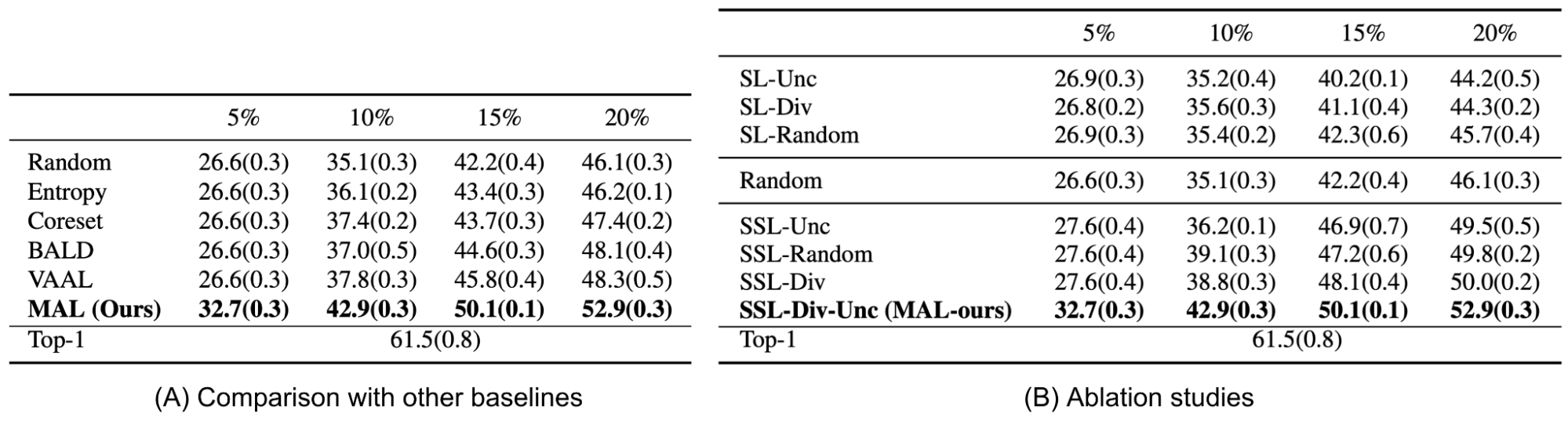
Experiments compared MAL against random, entropy, core-set, BALD, and VAAL baselines on image classification and segmentation tasks. The reported results appear quite strong.
CAL (Contrastive Active Learning; Margatina et al. 2021) aims to select contrastive examples. If two data points with different labels share similar network representations $\Phi(.)$, CAL treats them as contrastive examples. For a pair of contrastive examples $(\mathbf{x}_i, \mathbf{x}_j)$, they should satisfy:
Given an unlabeled sample $\mathbf{x}$, CAL proceeds as follows:
- Select the top $k$ nearest neighbors in model feature space among labeled samples, $\{(\mathbf{x}^l_i, y_i\}_{i=1}^M \subset \mathcal{X}$.
- Compute the KL divergence between the model output probabilities of $\mathbf{x}$ and each neighbor in $\{\mathbf{x}^l\}$. The contrastive score for $\mathbf{x}$ is the mean of these KL divergence values: $s(\mathbf{x}) = \frac{1}{M} \sum_{i=1}^M \text{KL}(p(y \vert \mathbf{x}^l_i | p(y \vert \mathbf{x}))$.
- Select samples with high contrastive scores for active learning.
Across a range of classification tasks, CAL’s experimental results are similar to the entropy baseline.
Measuring Representativeness
Core-sets Approach
A core-set is a concept from computational geometry, describing a small collection of points that approximates the shape of a larger point set. The approximation is captured by a geometric measure. In active learning, the goal is that a model trained on the core-set behaves comparably to a model trained on the full set of data points.
Sener & Savarese (2018) formulate active learning as a core-set selection problem. Suppose $N$ samples are available during training. In each active learning round $t$, a small subset is labeled, denoted $\mathcal{S}^{(t)}$. The learning objective admits the following upper bound, where the core-set loss is defined as the gap between the average empirical loss over labeled samples and the loss over the full dataset including unlabeled samples:
The active learning problem can then be reformulated as:
This is equivalent to the $k$-Center problem: select $b$ center points such that the maximum distance between any data point and its nearest center is minimized. The problem is NP-hard, and an approximate solution relies on a greedy algorithm.
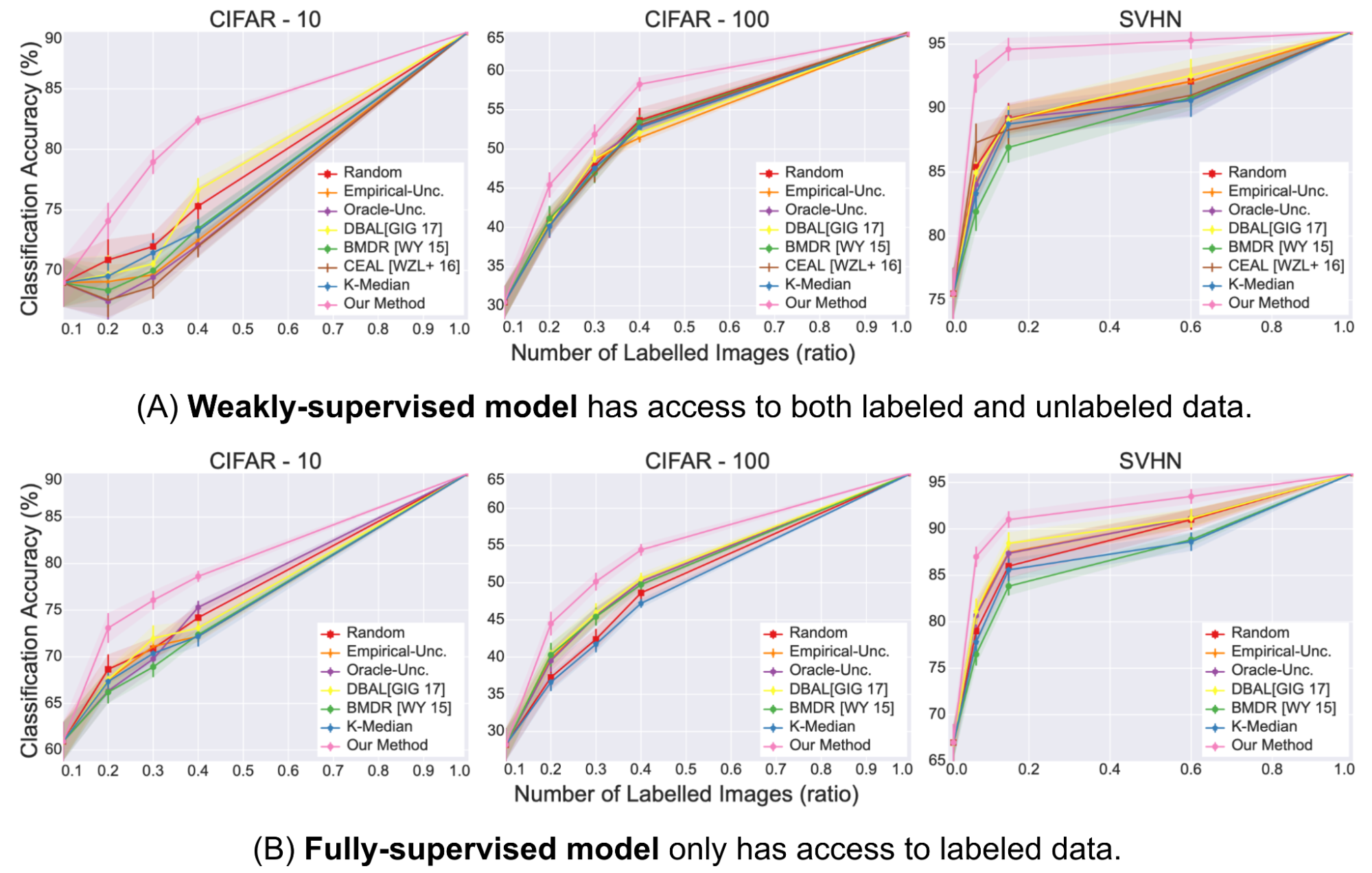
This approach performs well on image classification problems with a small number of classes. However, as the number of classes becomes large, or as data dimensionality increases (the “curse of dimensionality”), the core-set method becomes less effective (Sinha et al. 2019).
Since core-set selection is computationally costly, Coleman et al. (2020) tested using a weaker model (for example, a smaller architecture or a model that is not fully trained). They found empirically that using a weaker proxy model can substantially reduce the runtime of each repeated cycle of training models and selecting samples, while only minimally affecting the final error. This approach is referred to as SVP (Selection via Proxy).
Diverse Gradient Embedding
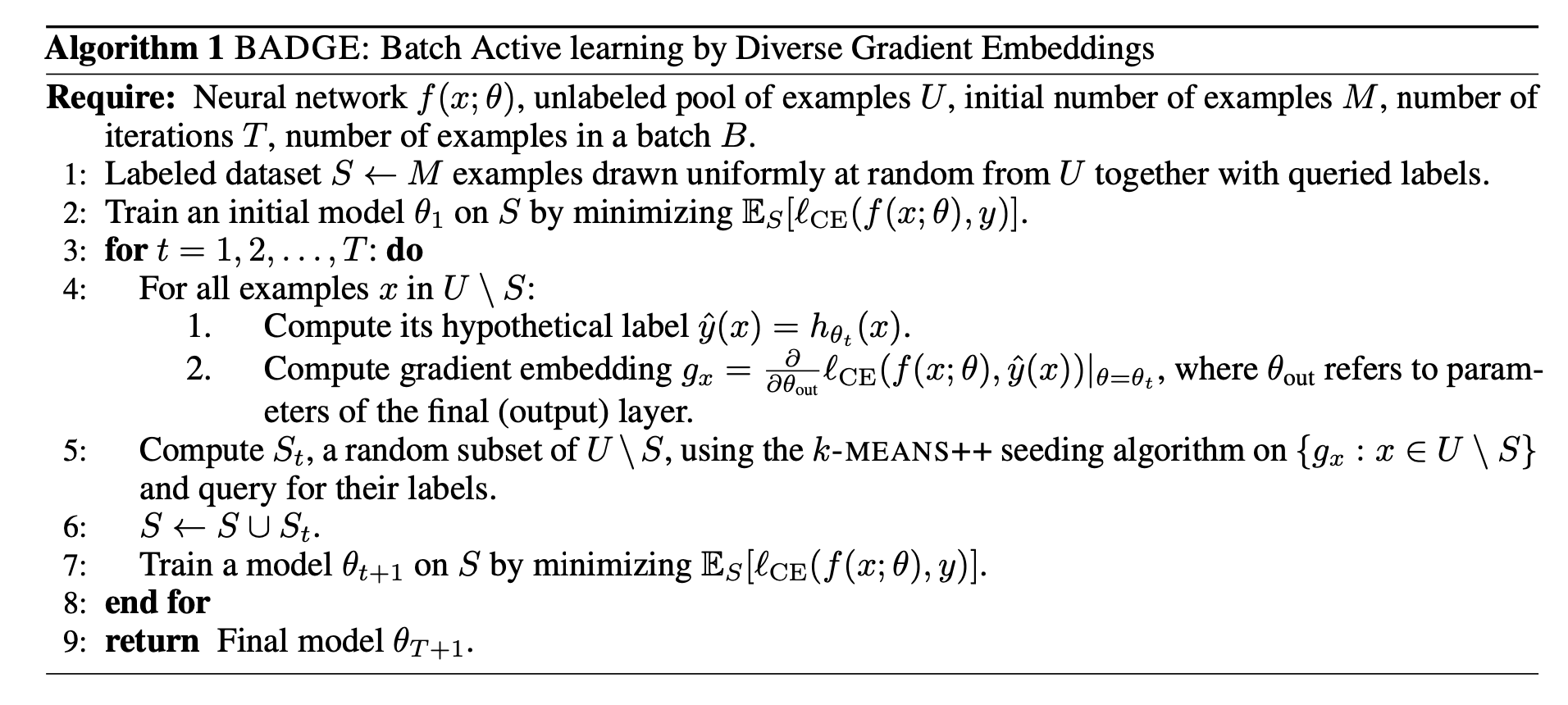
BADGE (Batch Active learning by Diverse Gradient Embeddings; Ash et al. 2020) simultaneously accounts for model uncertainty and data diversity in gradient space. It measures uncertainty via the gradient magnitude with respect to the network’s final layer, and it promotes diversity by selecting a varied set of samples that spans the gradient space.
- Uncertainty. Given an unlabeled sample $\mathbf{x}$, BADGE first computes the prediction $\hat{y}$ and the gradient $g_\mathbf{x}$ of the loss on $(\mathbf{x}, \hat{y})$ with respect to the last layer’s parameters. The authors observed that the norm of $g_\mathbf{x}$ provides a conservative estimate of the example’s influence on model learning, and that high-confidence samples tend to have gradient embeddings with small magnitude.
- Diversity. Given gradient embeddings for many samples, $g_\mathbf{x}$, BADGE runs $k$-means++ to sample data points accordingly.
Measuring Training Effects
Quantify Model Changes
Settles et al. (2008) proposed an active learning query strategy called EGL (Expected Gradient Length). Its key idea is to select samples that would induce the largest parameter update if their labels were available.
Let $\nabla \mathcal{L}(\theta)$ denote the gradient of the loss function with respect to the model parameters. Concretely, for an unlabeled sample $\mathbf{x}_i$, we compute the gradient under the assumption that its label is $y \in \mathcal{Y}$, $\nabla \mathcal{L}^{(y)}(\theta)$. Because the true label $y_i$ is unknown, EGL uses the model’s current belief to compute the expected gradient change:
BALD (Bayesian Active Learning by Disagreement; Houlsby et al. 2011) targets samples that maximize information gain about the model weights, which is equivalent to maximizing the reduction in expected posterior entropy.
The core intuition is to “seek $\mathbf{x}$ for which the model is marginally most uncertain about $y$ (high $H(y \vert \mathbf{x}, \mathcal{D})$), but for which individual settings of the parameters are confident (low $H(y \vert \mathbf{x}, \boldsymbol{\theta})$).” Put differently, each individual posterior draw is confident, but the set of draws reflects diverse opinions.
BALD was initially formulated for single-sample acquisition, and Kirsch et al. (2019) extended it to operate in batch mode.
Forgetting Events
To study whether neural networks tend to forget information they previously learned, Mariya Toneva et al. (2019) conducted an experiment in which they tracked the model’s prediction for each sample throughout training. They counted, for each sample, how often the prediction transitioned from correct to incorrect or from incorrect to correct. Based on these transitions, samples can be grouped as follows:
- Forgettable (redundant) samples: The class label changes across training epochs.
- Unforgettable samples: The class label assignment remains consistent across training epochs. Once learned, these samples are never forgotten.
The authors reported that many examples are unforgettable and, once learned, are never forgotten. In contrast, examples with noisy labels, or images with “uncommon” features (visually more complex to classify), are among the most frequently forgotten. Their experiments empirically showed that unforgettable examples can be removed safely without degrading model performance.
In their implementation, a forgetting event is counted only when the sample appears in the current training batch. That is, forgetting is measured across repeated presentations of the same example in successive mini-batches. The number of forgetting events per sample is fairly stable across random seeds, and forgettable examples are slightly more likely to be learned for the first time later in training. Forgetting events were also observed to transfer across the training process and across architectures.
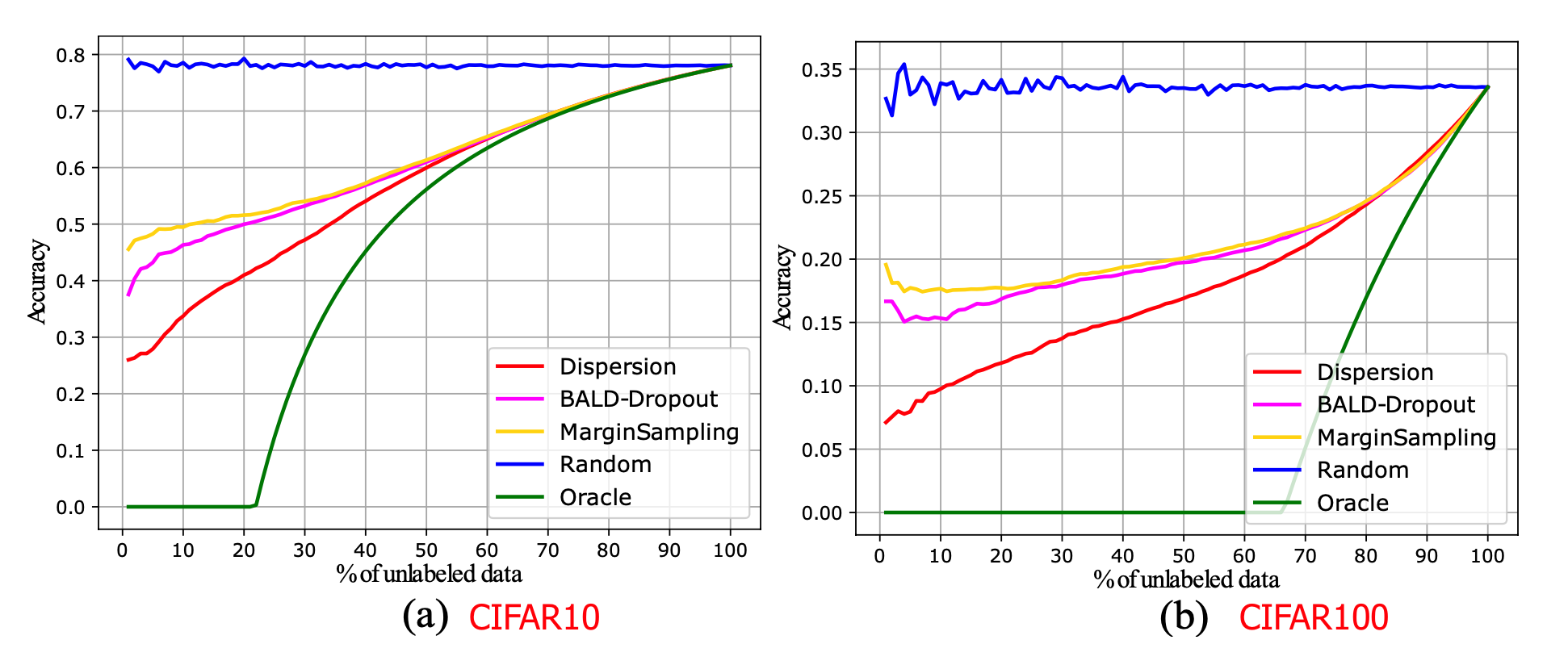
If we assume that prediction changes during training indicate model uncertainty, forgetting events could serve as an acquisition signal for active learning. However, for unlabeled samples the ground truth is unknown. To address this, Bengar et al. (2021) introduced a metric called label dispersion. Over training, let $c^*$ be the most frequently predicted label for input $\mathbf{x}$. Label dispersion measures the fraction of training steps in which the model does not assign $c^**$ to that sample:
In their implementation, dispersion is computed once per epoch. Label dispersion is low when the model consistently assigns the same label to a sample, and high when the prediction changes frequently. As illustrated in the figure below, label dispersion is correlated with network uncertainty.
Hybrid
In batch-mode active learning, controlling within-batch diversity is important. Suggestive Annotation (SA; Yang et al. 2017) is a two-stage hybrid approach designed to select samples that are both highly uncertain and highly representative. It estimates uncertainty using an ensemble of models trained on labeled data, and it uses core-sets to choose representative samples.
- First, SA selects the top $K$ images with high uncertainty scores to form a candidate pool $\mathcal{S}_c \subseteq \mathcal{S}_U$. Uncertainty is quantified as disagreement among multiple models trained via bootstrapping.
- Next, it selects a subset $\mathcal{S}_a \subseteq \mathcal{S}_c$ with the highest representativeness. Similarity between two inputs is approximated by the cosine similarity between their feature vectors. The representativeness of $\mathcal{S}_a$ for $\mathcal{S}_U$ captures how well $\mathcal{S}_a$ can represent all samples in $\mathcal{S}_u$, and is defined as:
Finding $\mathcal{S}_a \subseteq \mathcal{S}_c$ with $k$ data points that maximizes $F(\mathcal{S}_a, \mathcal{S}_u)$ is a generalized form of the maximum set cover problem. This optimization is NP-hard, and the best possible polynomial-time approximation is a straightforward greedy algorithm.
- Initialize $\mathcal{S}_a = \emptyset$ and $F(\mathcal{S}_a, \mathcal{S}_u) = 0$.
- Then, iteratively add $\mathbf{x}_i \in \mathcal{S}_c$ that maximizes $F(\mathcal{S}_a \cup I_i, \mathcal{S}_u)$ over $\mathcal{S}_a$, until $\mathcal{S}_s$ contains $k$ images.
Zhdanov (2019) follows a similar pipeline to SA, but in step 2 it uses $k$-means rather than a core-set method, with the candidate pool size set relative to the batch size. Given batch size $b$ and a constant $beta$ (between 10 and 50), the procedure is:
- Train a classifier on the labeled data;
- Compute the informativeness of every unlabeled example (for example, using uncertainty metrics);
- Prefilter the top $\beta b \geq b$ most informative examples;
- Cluster the $\beta b$ examples into $B$ clusters;
- Select $b$ distinct examples closest to the cluster centers for the current active learning round.
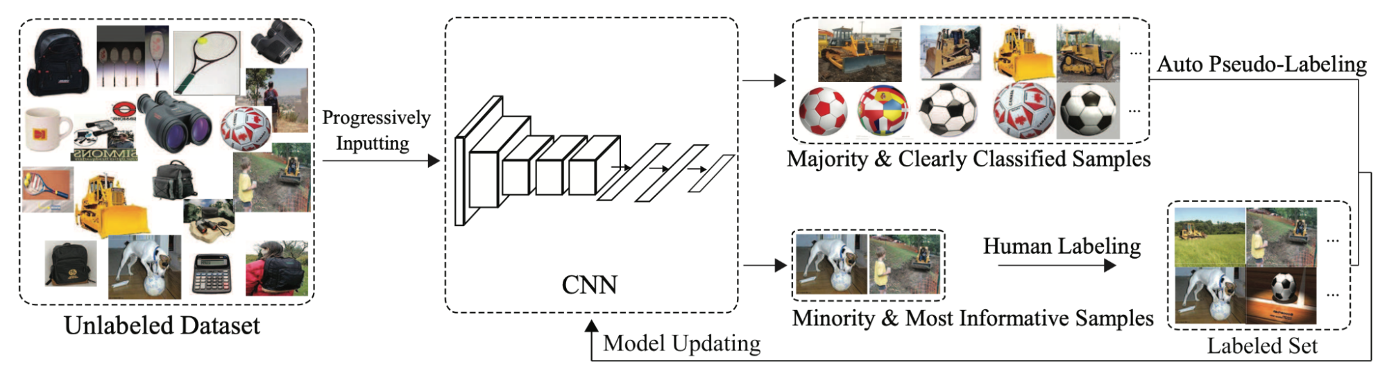
Active learning can also be combined with semi-supervised learning to reduce labeling cost. CEAL (Cost-Effective Active Learning; Yang et al. 2017) runs two processes in parallel:
- Select uncertain samples via active learning and obtain labels for them;
- Select samples with the most confident predictions and assign them pseudo labels. Prediction confidence is determined by whether prediction entropy falls below a threshold $\delta$. As the model improves over time, the threshold $\delta$ also decays over time.
Citation
Cited as:
Weng, Lilian. (Feb 2022). Learning with not enough data part 2: active learning. Lil’Log. https://lilianweng.github.io/posts/2022-02-20-active-learning/.
Or
@article{weng2022active,
  title   = "Learning with not Enough Data Part 2: Active Learning",
  author  = "Weng, Lilian",
  journal = "lilianweng.github.io",
  year    = "2022",
  month   = "Feb",
  url     = "https://lilianweng.github.io/posts/2022-02-20-active-learning/"
}
References
[1] Burr Settles. Active learning literature survey. University of Wisconsin, Madison, 52(55-66):11, 2010.
[2] https://jacobgil.github.io/deeplearning/activelearning
[3] Yang et al. “Cost-effective active learning for deep image classification” TCSVT 2016.
[4] Yarin Gal et al. “Dropout as a Bayesian Approximation: representing model uncertainty in deep learning.” ICML 2016.
[5] Blundell et al. “Weight uncertainty in neural networks (Bayes-by-Backprop)” ICML 2015.
[6] Settles et al. “Multiple-Instance Active Learning.” NIPS 2007.
[7] Houlsby et al. Bayesian Active Learning for Classification and Preference Learning." arXiv preprint arXiv:1112.5745 (2020).
[8] Kirsch et al. “BatchBALD: Efficient and Diverse Batch Acquisition for Deep Bayesian Active Learning.” NeurIPS 2019.
[9] Beluch et al. “The power of ensembles for active learning in image classification.” CVPR 2018.
[10] Sener & Savarese. “Active learning for convolutional neural networks: A core-set approach.” ICLR 2018.
[11] Donggeun Yoo & In So Kweon. “Learning Loss for Active Learning.” CVPR 2019.
[12] Margatina et al. “Active Learning by Acquiring Contrastive Examples.” EMNLP 2021.
[13] Sinha et al. “Variational Adversarial Active Learning” ICCV 2019
[14] Ebrahimiet al. “Minmax Active Learning” arXiv preprint arXiv:2012.10467 (2021).
[15] Mariya Toneva et al. “An empirical study of example forgetting during deep neural network learning.” ICLR 2019.
[16] Javad Zolfaghari Bengar et al. “When Deep Learners Change Their Mind: Learning Dynamics for Active Learning.” CAIP 2021.
[17] Yang et al. “Suggestive annotation: A deep active learning framework for biomedical image segmentation.” MICCAI 2017.
[18] Fedor Zhdanov. “Diverse mini-batch Active Learning” arXiv preprint arXiv:1901.05954 (2019).