The Transformer Family Version 2.0
Since my previous post on “The Transformer Family” (approximately three years ago), many improvements to Transformer architectures have been proposed. In this update, I performed a substantial refactor and expansion of that 2020 post: I reorganized the section hierarchy and strengthened many sections by incorporating more recent papers. Version 2.0 is a strict superset of the earlier version and is roughly twice as long. Notations Symbol Meaning $d$ The model size, hidden state dimension, positional encoding size. $h$ The number of heads in the multi-head attention layer. $L$ The segment length of the input sequence. $N$ The total number of attention layers in the model, excluding MoE. $\mathbf{X} \in \mathbb{R}^{L \times d}$ The input sequence, where each element has been mapped into an embedding vector of shape $d$, equal to the model size. $\mathbf{W}^k \in \mathbb{R}^{d \times d_k}$ The key weight matrix. $\mathbf{W}^q \in \mathbb{R}^{d \times d_k}$ The query weight matrix. $\mathbf{W}^v \in \mathbb{R}^{d \times d_v}$ The value weight matrix. Often we have $d_k = d_v = d$. $\mathbf{W}^k_i, \mathbf{W}^q_i \in \mathbb{R}^{d \times d_k/h}; \mathbf{W}^v_i \in \mathbb{R}^{d \times d_v/h}$ The per-head weight matrices. $\mathbf{W}^o \in \mathbb{R}^{d_v \times d}$ The output weight matrix. $\mathbf{Q} = \mathbf{X}\mathbf{W}^q \in \mathbb{R}^{L \times d_k}$ The query embedding inputs. $\mathbf{K} = \mathbf{X}\mathbf{W}^k \in \mathbb{R}^{L \times d_k}$ The key embedding inputs. $\mathbf{V} = \mathbf{X}\mathbf{W}^v \in \mathbb{R}^{L \times d_v}$ The value embedding inputs. $\mathbf{q}_i, \mathbf{k}_i \in \mathbb{R}^{d_k}, \mathbf{v}_i \in \mathbb{R}^{d_v}$ Row vectors in the query, key, and value matrices, $\mathbf{Q}$, $\mathbf{K}$, and $\mathbf{V}$. $S_i$ A collection of key positions for the $i$-th query $\mathbf{q}_i$ to attend to. $\mathbf{A} \in \mathbb{R}^{L \times L}$ The self-attention matrix between an input sequence of length $L$ and itself. $\mathbf{A} = \text{softmax}(\mathbf{Q}\mathbf{K}^\top / \sqrt{d_k})$. $a_{ij} \in \mathbf{A}$ The scalar attention score between query $\mathbf{q}_i$ and key $\mathbf{k}_j$. $\mathbf{P} \in \mathbb{R}^{L \times d}$ Position encoding matrix, where the $i$-th row $\mathbf{p}_i$ is the positional encoding for input $\mathbf{x}_i$. Transformer Basics The Transformer (referred to here as the “vanilla Transformer” to distinguish it from enhanced variants; Vaswani, et al., 2017) uses an encoder-decoder architecture, as is common in many NMT models. Later work showed that simplified Transformer variants can also deliver strong performance on language modeling tasks, such as encoder-only BERT and decoder-only GPT.
· 45 min read · Curated and presented by Arthur Sedek
Since my previous post, “The Transformer Family”, published about three years ago, many improvements to the Transformer architecture have been introduced. Here, I have thoroughly refactored and expanded that 2020 article by reorganizing the section hierarchy and updating numerous sections with more recent papers. Version 2.0 is a superset of the earlier version and is roughly twice as long.
Notations
| Symbol | Meaning |
|---|---|
| $d$ | The model size / hidden state dimension / positional encoding size. |
| $h$ | The number of heads in multi-head attention layer. |
| $L$ | The segment length of input sequence. |
| $N$ | The total number of attention layers in the model; not considering MoE. |
| $\mathbf{X} \in \mathbb{R}^{L \times d}$ | The input sequence where each element has been mapped into an embedding vector of shape $d$, same as the model size. |
| $\mathbf{W}^k \in \mathbb{R}^{d \times d_k}$ | The key weight matrix. |
| $\mathbf{W}^q \in \mathbb{R}^{d \times d_k}$ | The query weight matrix. |
| $\mathbf{W}^v \in \mathbb{R}^{d \times d_v}$ | The value weight matrix. Often we have $d_k = d_v = d$. |
| $\mathbf{W}^k_i, \mathbf{W}^q_i \in \mathbb{R}^{d \times d_k/h}; \mathbf{W}^v_i \in \mathbb{R}^{d \times d_v/h}$ | The weight matrices per head. |
| $\mathbf{W}^o \in \mathbb{R}^{d_v \times d}$ | The output weight matrix. |
| $\mathbf{Q} = \mathbf{X}\mathbf{W}^q \in \mathbb{R}^{L \times d_k}$ | The query embedding inputs. |
| $\mathbf{K} = \mathbf{X}\mathbf{W}^k \in \mathbb{R}^{L \times d_k}$ | The key embedding inputs. |
| $\mathbf{V} = \mathbf{X}\mathbf{W}^v \in \mathbb{R}^{L \times d_v}$ | The value embedding inputs. |
| $\mathbf{q}_i, \mathbf{k}_i \in \mathbb{R}^{d_k}, \mathbf{v}_i \in \mathbb{R}^{d_v}$ | Row vectors in query, key, value matrices, $\mathbf{Q}$, $\mathbf{K}$ and $\mathbf{V}$. |
| $S_i$ | A collection of key positions for the $i$-th query $\mathbf{q}_i$ to attend to. |
| $\mathbf{A} \in \mathbb{R}^{L \times L}$ | The self-attention matrix between a input sequence of lenght $L$ and itself. $\mathbf{A} = \text{softmax}(\mathbf{Q}\mathbf{K}^\top / \sqrt{d_k})$. |
| $a_{ij} \in \mathbf{A}$ | The scalar attention score between query $\mathbf{q}_i$ and key $\mathbf{k}_j$. |
| $\mathbf{P} \in \mathbb{R}^{L \times d}$ | position encoding matrix, where the $i$-th row $\mathbf{p}_i$ is the positional encoding for input $\mathbf{x}_i$. |
Transformer Basics
The Transformer model (referred to here as the “vanilla Transformer” to distinguish it from later enhanced variants; Vaswani, et al., 2017) uses an encoder-decoder architecture, a standard design in many NMT systems. Subsequent simplified Transformer variants were later shown to perform very well on language modeling tasks, including encoder-only models such as BERT and decoder-only models such as GPT.
Attention and Self-Attention
Attention is a neural network mechanism that enables a model to form predictions by selectively focusing on a given set of data. The degree of attention is represented by learned weights, and the resulting output is typically computed as a weighted average.
Self-attention is an attention mechanism in which the model predicts one part of a data sample using other parts of the observation from the same sample. Conceptually, it is closely related to non-local means. Note also that self-attention is permutation-invariant, meaning it operates on sets.
Attention and self-attention can be implemented in multiple ways. In the Transformer (Vaswani et al., 2017), the core primitive is scaled dot-product attention. Given a query matrix $\mathbf{Q}$, a key matrix $\mathbf{K}$, and a value matrix $\mathbf{V}$, the output is computed as a weighted sum of the value vectors. The weight assigned to each value position is determined by the dot-product between the query and the corresponding key:
For a query and a key vector $\mathbf{q}_i, \mathbf{k}_j \in \mathbb{R}^d$ (row vectors from the query and key matrices), the corresponding scalar score is:
where $\mathcal{S}_i$ denotes the set of key positions that the $i$-th query is allowed to attend to.
For other attention variants, see my earlier post for other types of attention.
Multi-Head Self-Attention
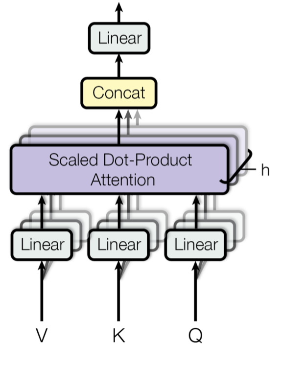
The multi-head self-attention module is a central building block in the Transformer. Instead of computing attention a single time, the multi-head mechanism partitions the input into smaller subspaces and computes scaled dot-product attention in parallel within each subspace. The resulting attention outputs are then concatenated and passed through a linear transformation to produce the desired dimensions.
Here, $[.;.]$ denotes concatenation. $\mathbf{W}^q_i, \mathbf{W}^k_i \in \mathbb{R}^{d \times d_k/h}, \mathbf{W}^v_i \in \mathbb{R}^{d \times d_v/h}$ are learned weight matrices that project input embeddings of size $L \times d$ into query, key, and value matrices. $\mathbf{W}^o \in \mathbb{R}^{d_v \times d}$ is the learned output projection. All weights are learned during training.
Encoder-Decoder Architecture
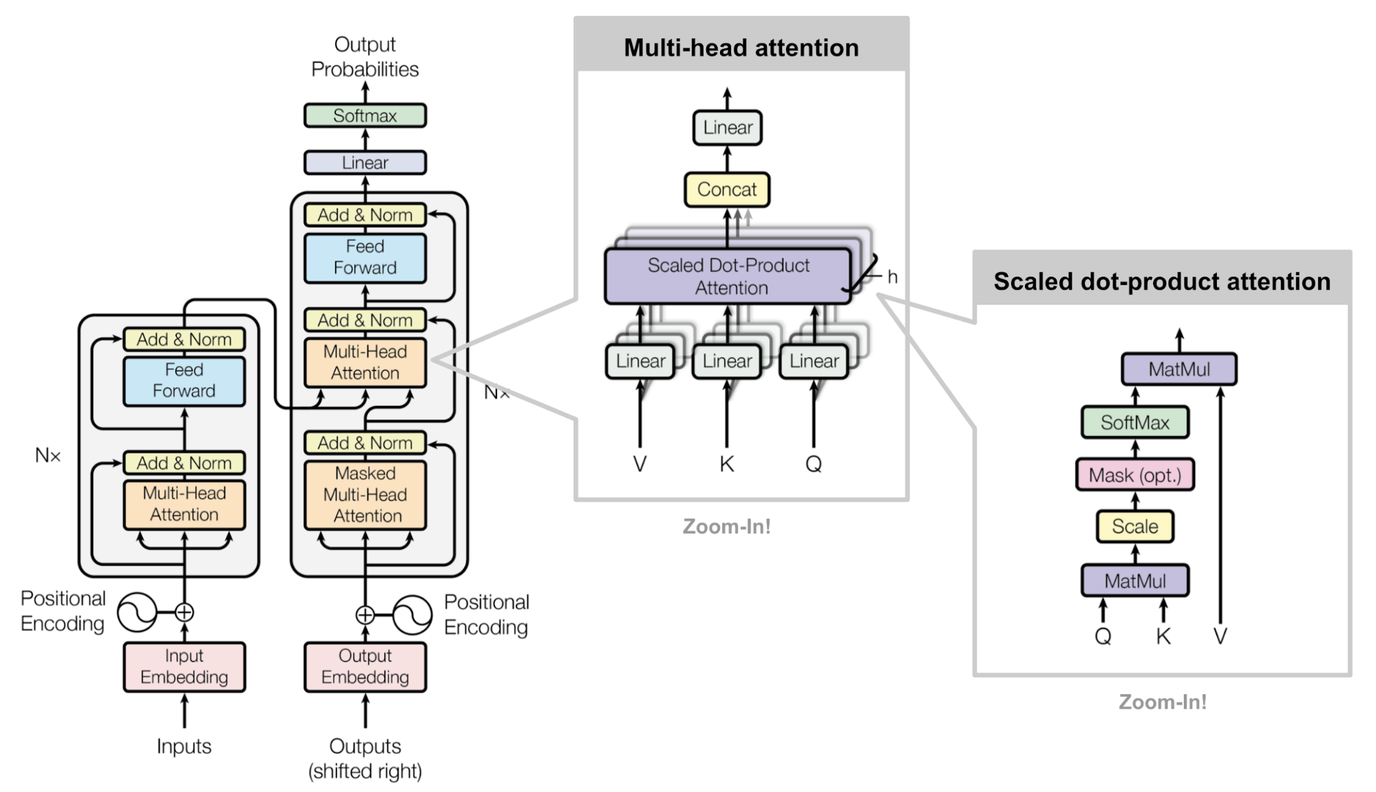
The encoder produces an attention-based representation that can locate specific information within a large context. It is composed of a stack of 6 identical modules, and each module contains two submodules: a multi-head self-attention layer and a point-wise fully connected feed-forward network. “Point-wise” indicates that the same linear transformation (with shared weights) is applied independently to each sequence position. This can also be interpreted as a convolutional layer with filter size 1. Each submodule is wrapped with a residual connection and layer normalization. All submodules produce outputs of the same dimensionality $d$.
The Transformer decoder retrieves information from the encoder representation. Its structure closely mirrors the encoder, except that each repeated module in the decoder contains two multi-head attention submodules rather than one. The first multi-head attention submodule is masked so that a position cannot attend to future positions.
Positional Encoding
Because self-attention is permutation-invariant, the model requires an appropriate positional encoding mechanism to inject order information. The positional encoding $\mathbf{P} \in \mathbb{R}^{L \times d}$ is defined to have the same dimensionality as the input embeddings, so it can be added directly to the input. The vanilla Transformer considered two encoding approaches:
Sinusoidal Positional Encoding
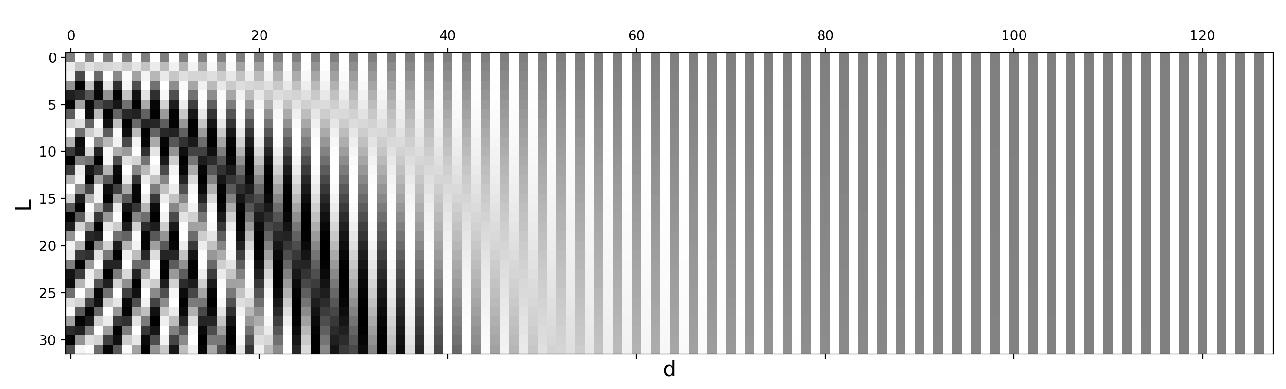
Sinusoidal positional encoding is defined as follows. Given the token position $i=1,\dots,L$ and the dimension $\delta=1,\dots,d$:
With this design, each positional-encoding dimension corresponds to a sinusoid of a different wavelength, spanning $2\pi$ to $10000 \cdot 2\pi$ across dimensions.
Learned Positional Encoding
Learned positional encoding assigns each element a learned column vector representing its absolute position (Gehring, et al. 2017). Furthermore, this encoding can be learned separately for each layer (Al-Rfou et al. 2018).
Relative Position Encoding
Shaw et al. (2018)) incorporated relative positional information into $\mathbf{W}^k$ and $\mathbf{W}^v$. The maximum relative position is clipped to a maximum absolute value of $k$, and this clipping allows the model to generalize to unseen sequence lengths. As a result, $2k + 1$ unique edge labels are used, and we denote $\mathbf{P}^k, \mathbf{P}^v \in \mathbb{R}^{2k+1}$ as the learnable relative position representations.
Transformer-XL (Dai et al., 2019) introduced a form of relative positional encoding via a reparameterization of the query and key dot-product. To keep positional information consistent across segments, Transformer-XL encodes relative positions rather than absolute ones, since knowing the position offset can be sufficient for accurate prediction, that is, $i-j$, between a key vector $\mathbf{k}_{\tau, j}$ and its query $\mathbf{q}_{\tau, i}$.
If we omit the scalar $1/\sqrt{d_k}$ and the softmax normalization term, while including positional encodings, the attention score between the query at position $i$ and the key at position $j$ can be written as:
Transformer-XL then reparameterizes these four terms as:
- Replace $\mathbf{p}_j$ with the relative positional encoding $\mathbf{r}_{i-j} \in \mathbf{R}^{d}$;
- Replace $\mathbf{p}_i\mathbf{W}^q$ with two trainable parameters, $\mathbf{u}$ (content) and $\mathbf{v}$ (location), used in two separate terms;
- Split $\mathbf{W}^k$ into two matrices: $\mathbf{W}^k_E$ for content information and $\mathbf{W}^k_R$ for location information.
Rotary Position Embedding
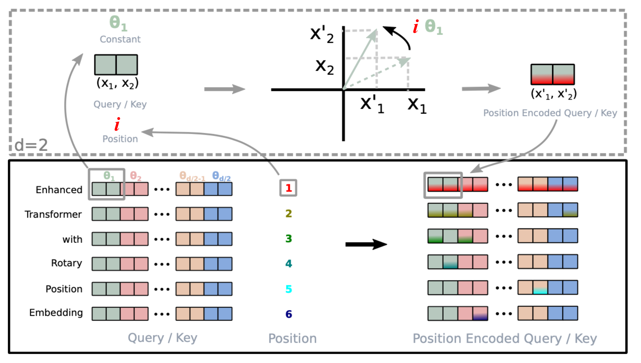
Rotary position embedding (RoPE; Su et al. 2021) represents absolute position using a rotation matrix. It multiplies the key and value matrices in every attention layer by this matrix, thereby injecting relative positional information at every layer.
When encoding relative positional information into the inner product between the $i$-th key and the $j$-th query, the goal is to express the inner product as a function only of the relative position $i-j$. RoPE uses Euclidean rotation and frames relative position embedding as rotating the feature matrix by an angle proportional to its position index.
Given a vector $\mathbf{z}$, a counterclockwise rotation by $\theta$ can be obtained by multiplying by a rotation matrix, producing $R\mathbf{z}$, where the rotation matrix $R$ is:
To generalize to higher-dimensional spaces, RoPE divides the $d$-dimensional space into $d/2$ subspaces and constructs a rotation matrix $R$ of size $d \times d$ for the token at position $i$:
where the paper uses $\Theta = {\theta_i = 10000^{-2(i−1)/d}, i \in [1, 2, …, d/2]}$. Note that this is essentially equivalent to sinusoidal positional encoding, but expressed in terms of a rotation matrix.
Both key and query matrices incorporate positional information by multiplying by the rotation matrix:
Longer Context
For Transformer models, the maximum input sequence length at inference time is bounded by the context length used during training. A naive increase in context length significantly increases both time ($\mathcal{O}(L^2d)$) and memory ($\mathcal{O}(L^2)$) usage and may be infeasible under hardware constraints.
This section describes several architectural improvements that better support long-context inference, such as adding memory, designing mechanisms for improved context extrapolation, or introducing recurrence.
Context Memory
The vanilla Transformer has a fixed and limited attention span. During each update step, it can attend only to elements within the same segment, and information cannot flow across separate fixed-length segments. This context segmentation creates several problems:
- The model cannot represent very long-term dependencies.
- Predicting the first few tokens in each segment is difficult because the available context is absent or very limited.
- Evaluation becomes expensive. When the segment window shifts to the right by one, the new segment must be recomputed from scratch, even though many tokens overlap.
Transformer-XL (Dai et al., 2019; “XL” stands for “extra long”) changes the architecture to reuse hidden states across segments by introducing an additional memory. It establishes a recurrent connection between segments by continually incorporating hidden states from preceding segments.
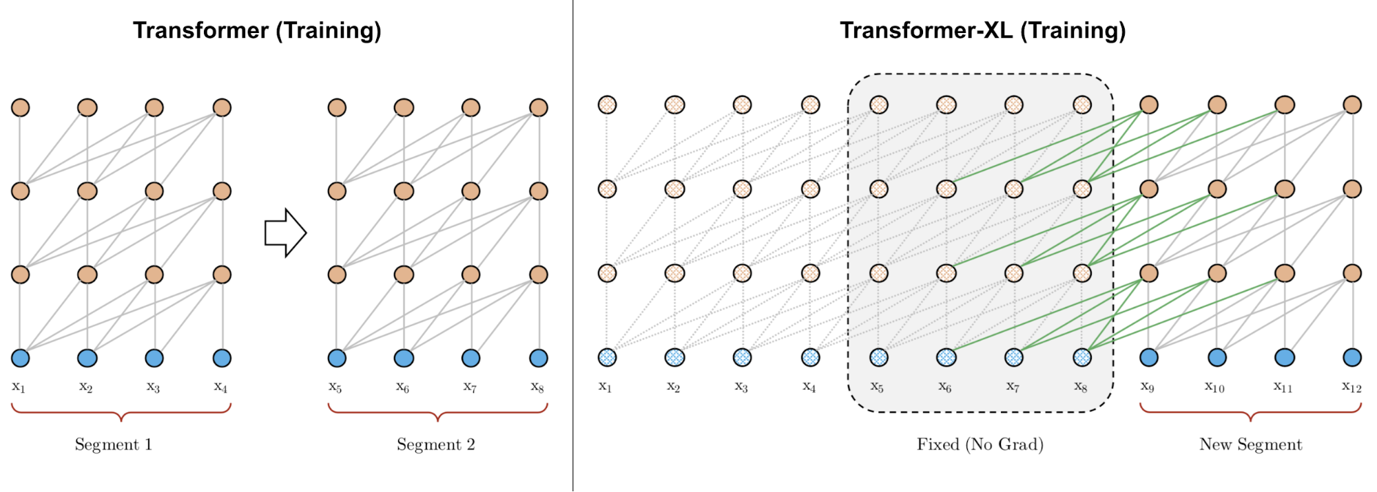
Let the hidden state in the $n$-th layer for the $(\tau + 1)$-th segment be denoted as $\mathbf{h}_{\tau+1}^{(n)} \in \mathbb{R}^{L \times d}$. In addition to depending on the hidden state of the last layer for the same segment $\mathbf{h}_{\tau+1}^{(n-1)}$, it also depends on the hidden state of the same layer from the previous segment $\mathbf{h}_{\tau}^{(n)}$. By incorporating previous hidden states, the model extends its attention span much further into the past, across multiple segments.
Note that keys and values depend on the extended hidden states, while queries use only the hidden states at the current step. The concatenation operation $[. \circ .]$ is performed along the sequence-length dimension. Transformer-XL also requires relative positional encoding, because if absolute positions were encoded, both the previous and current segments would receive the same encoding, which is undesirable.
Compressive Transformer (Rae et al. 2019) extends Transformer-XL by compressing past memories to support longer sequences. It explicitly introduces memory slots of size $m_m$ per layer to store past activations from that layer and preserve long-range context. When past activations become sufficiently old, they are compressed and stored in an additional compressed memory of size $m_{cm}$ per layer.
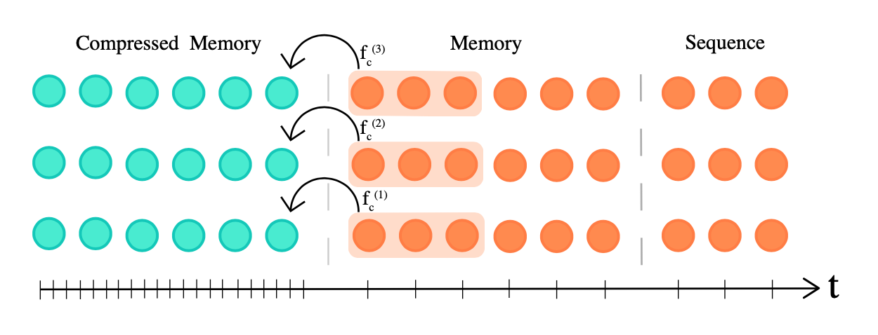
Both the memory and compressed memory are FIFO queues. Given a model context length $L$, the compression function with compression rate $c$ is defined as $f_c: \mathbb{R}^{L \times d} \to \mathbb{R}^{[\frac{L}{c}] \times d}$, mapping the $L$ oldest activations to $[\frac{L}{c}]$ compressed memory elements. Several compression functions are possible:
- Max/mean pooling with kernel and stride size $c$;
- 1D convolution with kernel and stride size $c$ (requires learning additional parameters);
- Dilated convolution (requires learning additional parameters). In their experiments, convolution-based compression performs best on the
EnWik8dataset; - Most used memories.
Compressive Transformer adds two extra training losses:
-
Auto-encoding loss (a lossless compression objective), which measures how accurately original memories can be reconstructed from compressed memories
$ \mathcal{L}_{ac} = \| \textbf{old_mem}^{(i)} - g(\textbf{new_cm}^{(i)}) \|_2 $where $g: \mathbb{R}^{[\frac{L}{c}] \times d} \to \mathbb{R}^{L \times d}$ inverts the compression function $f$. -
Attention-reconstruction loss (a lossy objective), which reconstructs content-based attention over memory versus compressed memory and minimizes the discrepancy:
$ \mathcal{L}_{ar} = \|\text{attn}(\mathbf{h}^{(i)}, \textbf{old_mem}^{(i)}) − \text{attn}(\mathbf{h}^{(i)}, \textbf{new_cm}^{(i)})\|_2 $
Transformer-XL with memory size $m$ has a maximum temporal range of $m \times N$, where $N$ is the number of model layers, and an attention cost of $\mathcal{O}(L^2 + Lm)$. In contrast, Compressive Transformer achieves a temporal range of $(m_m + c \cdot m_{cm}) \times N$ with attention cost $\mathcal{O}(L^2 + L(m_m + m_{cm}))$. A larger compression rate $c$ provides a better tradeoff between temporal range and attention cost.
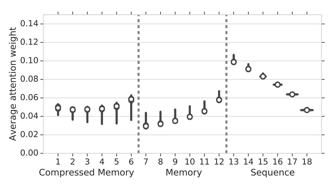
Attention weights, from oldest to newest, are stored across three locations: compressed memory → memory → causally masked sequence. In the experiments, attention weights increased from the oldest activations stored in regular memory to activations stored in compressed memory, suggesting that the network learns to preserve salient information.
Non-Differentiable External Memory
$k$NN-LM (Khandelwal et al. 2020) augments a pretrained LM with a separate $k$NN model by linearly interpolating the next-token probabilities produced by the two models. The $k$NN model is built on an external key-value store that can hold a large pre-training dataset or an OOD dataset introduced later. The datastore is preprocessed to store a large collection of (LM embedding representation of context, next token) pairs, and nearest-neighbor retrieval is performed in the LM embedding space. Because the datastore can be extremely large, fast dense vector search libraries such as FAISS or ScaNN are needed. Indexing is performed once, and it is straightforward to implement parallelism at inference time.
During inference, the next-token probability is computed as a weighted sum of the two predictions:
where $\mathcal{N}$ is a set of nearest-neighbor datapoints retrieved by $k$NN, and $d(., .)$ is a distance function such as L2 distance.
Based on the experiments, larger datastore sizes or larger $k$ are associated with improved perplexity. The weighting scalar $\lambda$ must be tuned, but it is generally expected to be larger for out-of-domain data than for in-domain data, and a larger datastore can support a larger $\lambda$.
SPALM (Adaptive semiparametric language models; Yogatama et al. 2021) combines (1) Transformer-XL-style memory of hidden states from external context as short-term memory and (2) $k$NN-LM-style key-value storage as long-term memory.
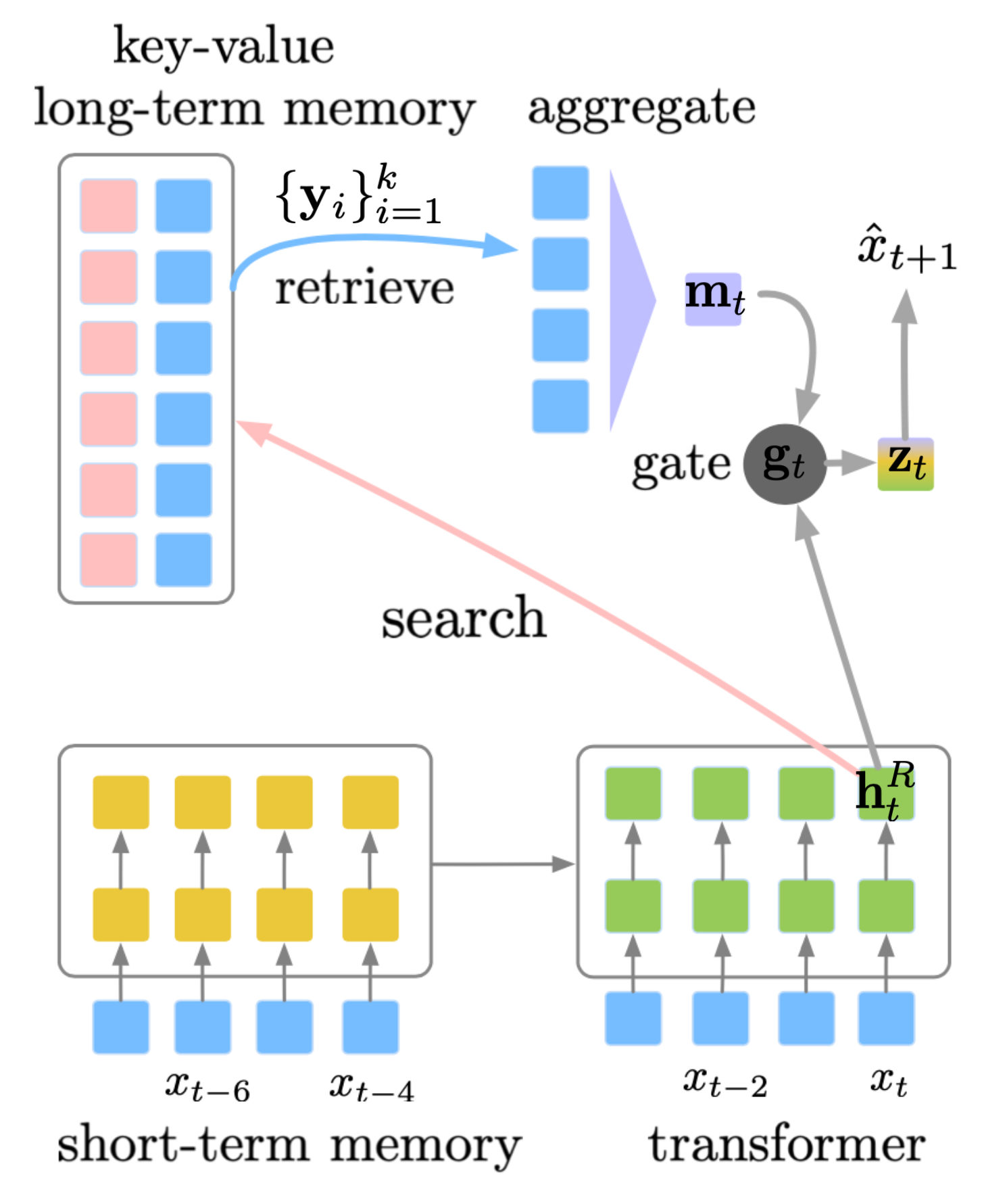
SPALM runs $k$NN search to retrieve $k$ tokens with the most relevant context. For each retrieved token, we obtain the same embedding representation produced by a pretrained LM, denoted as $\{\mathbf{y}_i\}_{i=1}^k$. The gating mechanism first aggregates the retrieved token embeddings using a simple attention layer, with $\mathbf{h}^R_t$ (the hidden state of token $x_t$ at layer $R$) serving as the query. It then learns a gating parameter $\mathbf{g}_t$ to balance local information $\mathbf{h}^R_t$ against long-term information $\mathbf{m}_t$.
Here, $\mathbf{w}_g$ is a parameter vector to be learned, $\sigma(.)$ is the sigmoid function, and $\mathbf{W}$ is the word embedding matrix shared by both input and output tokens. Unlike $k$NN-LM, the authors did not find nearest-neighbor distance to be useful when aggregating retrieved tokens.
During training, the key representations stored in long-term memory remain fixed (they are produced by a pretrained LM), whereas the value encoder, that is, the word embedding matrix, is updated.
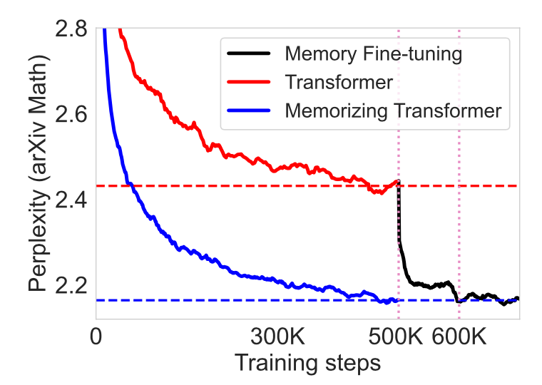
Memorizing Transformer (Wu et al. 2022) introduces a $k$NN-augmented attention layer near the top of a decoder-only Transformer stack. This specialized layer maintains a Transformer-XL-style FIFO cache containing past key-value pairs.
The same QKV values are used for both local attention and $k$NN mechanisms. The $k$NN lookup returns the top-$k$ (key, value) pairs for each query in the input sequence, and these retrieved pairs are then processed through the self-attention stack to compute a weighted average of retrieved values. The two attention types are merged using a learnable, per-head gating parameter. To avoid large distributional shifts in value magnitude, both keys and values in the cache are normalized.
Findings reported from experiments with Memorizing Transformer include the following:
- In some experiments, training with a small memory and then fine-tuning with a larger memory performed better than training with a large memory from scratch.
- A smaller Memorizing Transformer with only 8k tokens in memory can match the perplexity of a larger vanilla Transformer with 5X more trainable parameters.
- Increasing the size of external memory produced consistent gains up to a size of 262K.
- A non-memory transformer can be fine-tuned to use memory.
Distance-Enhanced Attention Scores
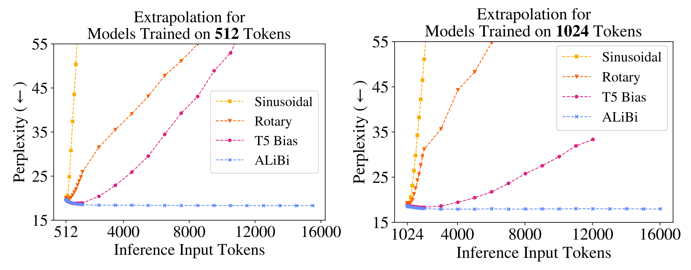
Distance Aware Transformer (DA-Transformer; Wu, et al. 2021) and Attention with Linear Biases (ALiBi; Press et al. 2022) are motivated by the same core idea. To encourage extrapolation to longer contexts than those seen during training, we can explicitly incorporate positional information into each attention score by using the distance between key and query tokens.
Note that the default positional encoding in the vanilla Transformer only injects positional information into the input sequence. In contrast, later mechanisms modify attention scores at every layer, such as rotary position embedding, and these approaches take a form that is closely related to distance-enhanced attention scores.
DA-Transformer (Wu, et al. 2021) multiplies attention scores in each layer by a learnable bias defined as a function of the distance between key and query. Different attention heads use different parameters, allowing them to express distinct preferences for short-term versus long-term context. Given two positions, $i, j$, DA-Transformer applies the following weighting function to modify the self-attention score:
In this formulation, $\alpha_i$ is a learnable parameter that weights relative distance differently per head, with the head indexed by the superscript $^{(i)}$. $\beta_i$ is a learnable parameter that controls the upper bound and ascending slope with respect to distance for the $i$-th attention head. The weighting function $f(.)$ is constructed to satisfy the following properties: (1) $f(0)=1$; (2) $f(\mathbf{R}^{(i)}) = 0$ when $\mathbf{R}^{(i)} \to -\infty$; (3) $f(\mathbf{R}^{(i)})$ is bounded when $\mathbf{R}^{(i)} \to +\infty$; (4) the scale is tunable; and (5) the function is monotonic. The additional time complexity introduced by $f(\mathbf{R}^{(i)})$ is $\mathcal{O}(L^2)$, which is small relative to the self-attention time complexity $\mathcal{O}(L^2 d)$. The additional memory usage is minimal, approximately $\mathcal{O}(2h)$.
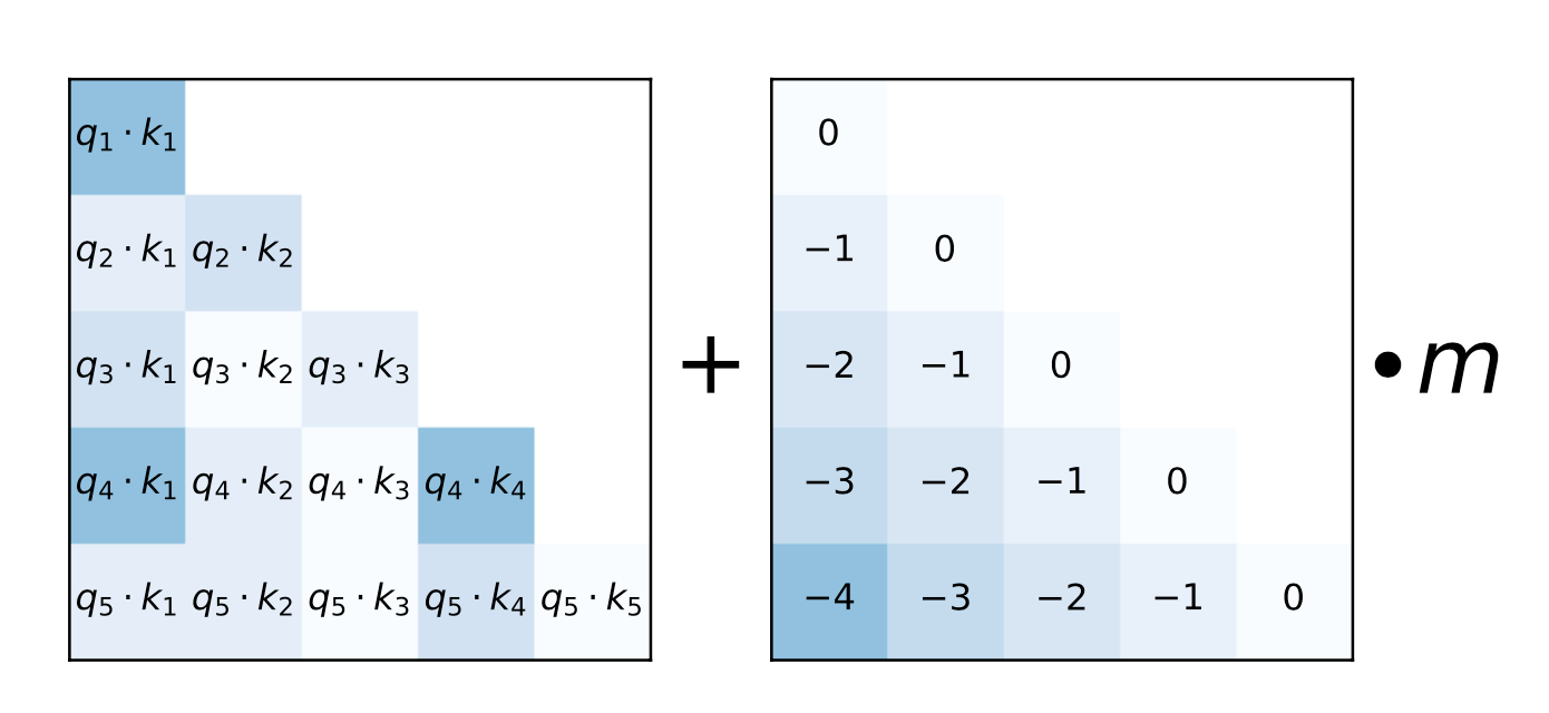
Rather than using multipliers, ALiBi (Press et al. 2022) adds a constant bias term to query-key attention scores that is proportional to pairwise distances. This bias induces a strong recency preference by penalizing keys that are far away. Different heads increase penalties at different rates. $ \text{softmax}(\mathbf{q}_i \mathbf{K}^\top + \alpha_i \cdot [0, -1, -2, \dots, -(i-1)]) $ where $\alpha_i$ is a head-specific weighting scalar. In contrast to DA-Transformer, $\alpha_i$ is not learned; it is fixed as a geometric sequence. For example, with 8 heads, ${\alpha_i} = {\frac{1}{2}, \frac{1}{2^2}, \dots, \frac{1}{2^8}}$. The overall motivation closely matches what relative positional encoding is designed to address.
Using ALiBi, Press et al. (2022) trained a 1.3B-parameter model with a context length of 1024 during training and extrapolated to 2046 during inference.
Make it Recurrent
Universal Transformer (Dehghani, et al. 2019) integrates Transformer self-attention with an RNN-style recurrence mechanism, aiming to combine the long-term global receptive field of Transformers with learned inductive biases from RNNs. Instead of using a fixed number of layers, the Universal Transformer dynamically determines the number of steps using adaptive computation time. When the number of steps is fixed, a Universal Transformer is equivalent to a multi-layer Transformer whose layers share parameters.
At a high level, the Universal Transformer can be interpreted as a recurrent function that learns a hidden-state representation for each token. This recurrent function evolves in parallel across token positions, while information is exchanged across positions via self-attention.
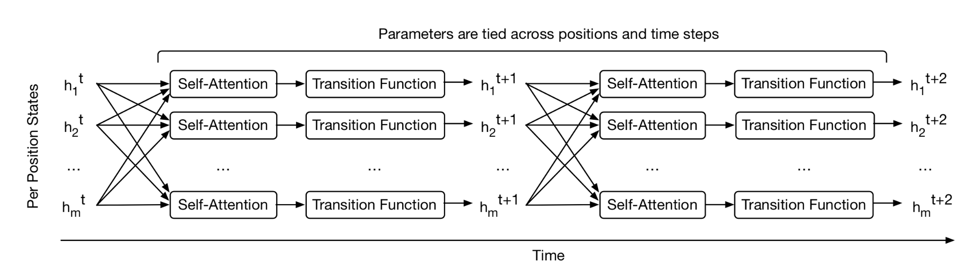
Given an input sequence of length $L$, the Universal Transformer iteratively updates the representation $\mathbf{h}^t \in \mathbb{R}^{L \times d}$ at step $t$ for an adjustable number of steps. At step 0, $\mathbf{h}^0$ is initialized to match the input embedding matrix. All positions are processed in parallel by multi-head self-attention and then passed through a recurrent transition function.
In this equation, $\text{Transition}(.)$ is either a separable convolution or a fully connected neural network composed of two position-wise (that is, applied to each row of $\mathbf{A}^t$ independently) affine transformations plus one ReLU.
The positional encoding $\mathbf{P}^t$ uses a sinusoidal position signal with an additional time dimension:
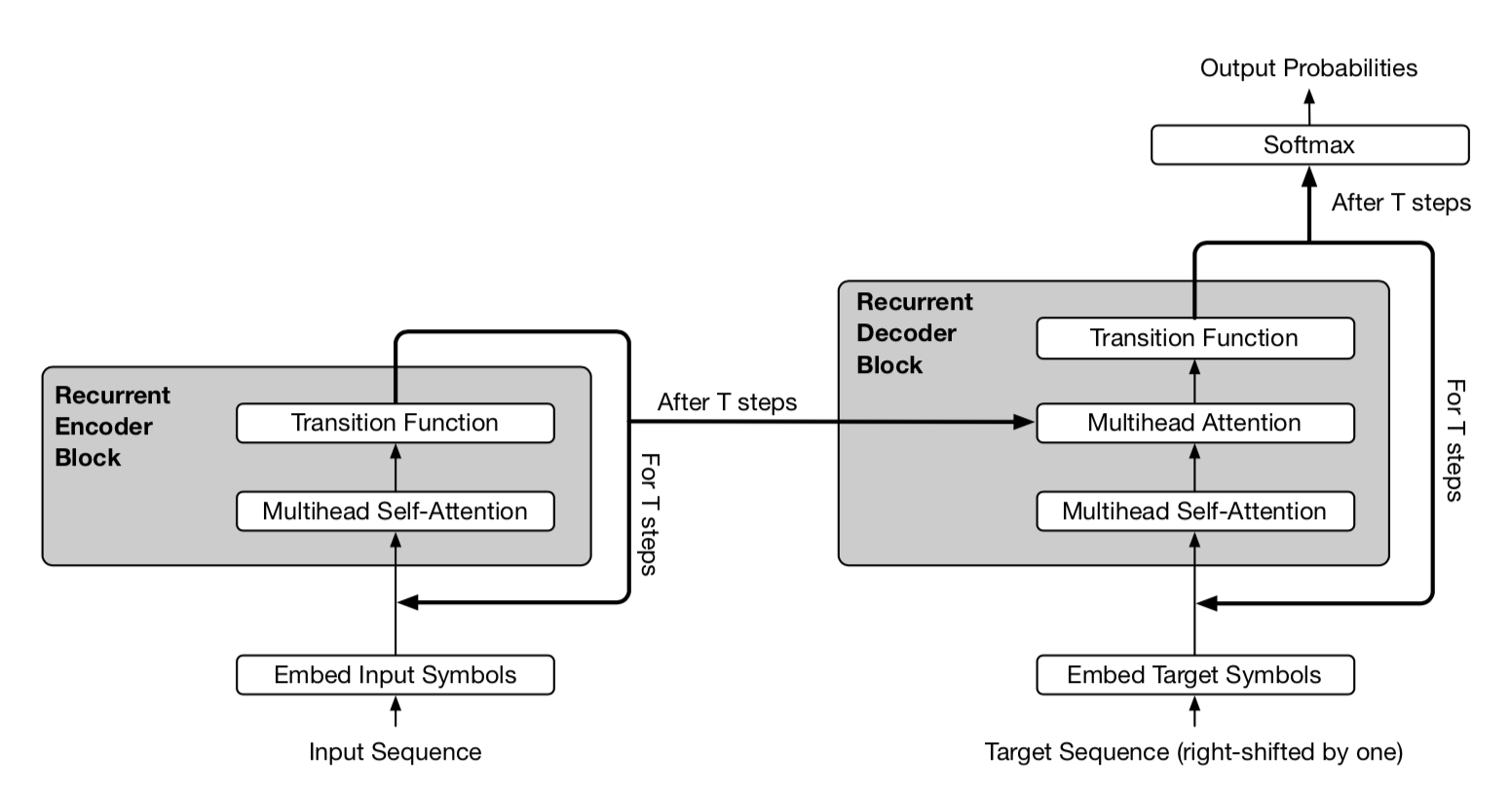
In the adaptive variant of the Universal Transformer, the number of recurrent steps $T$ is determined dynamically using ACT. Each position is equipped with its own ACT halting mechanism. Once a per-token recurrent block halts, it no longer receives recurrent updates; instead, it copies its current value forward to the next step until all blocks have halted or the model reaches a maximum step limit.
Adaptive Modeling
Adaptive modeling refers to mechanisms that adjust the amount of computation based on the input. For example, some tokens may only require local information and therefore benefit from a shorter attention span, while other tokens may be easier to predict and do not need to traverse the full attention stack.
Adaptive Attention Span
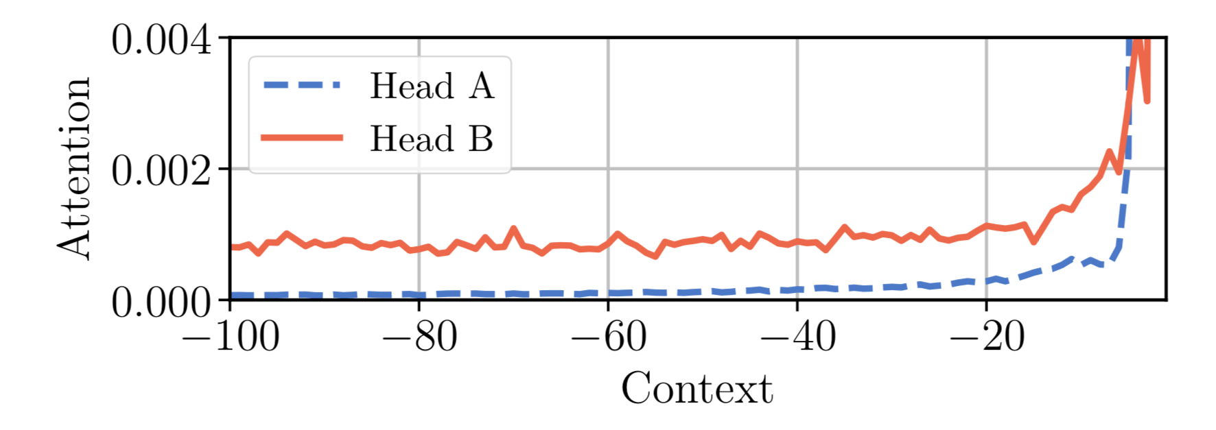
A key strength of the Transformer is its ability to capture long-term dependencies. However, depending on the context, the model may prefer to attend farther back in some cases than in others, and one attention head may exhibit a different pattern from another. If the attention span could flexibly adapt its length, attending farther back only when necessary, the model could reduce both computation and memory costs while supporting a larger maximum context length.
This motivation underlies Adaptive Attention Span. Sukhbaatar et al (2019) proposed a self-attention mechanism that learns an optimal attention span. They hypothesized that different heads may allocate attention differently within the same context window (see Fig. 14), and therefore trained the optimal span separately for each head.
For the $i$-th token, we compute attention weights between this token and other keys within an attention span of size $s$:
A soft mask function $m_z$ is introduced to enforce an effectively adjustable attention span by mapping the query-key distance to a value in [0, 1]. $m_z$ is parameterized by $z \in [0, s]$, and $z$ is learned:
where $R$ is a hyperparameter that controls the softness of $m_z$.
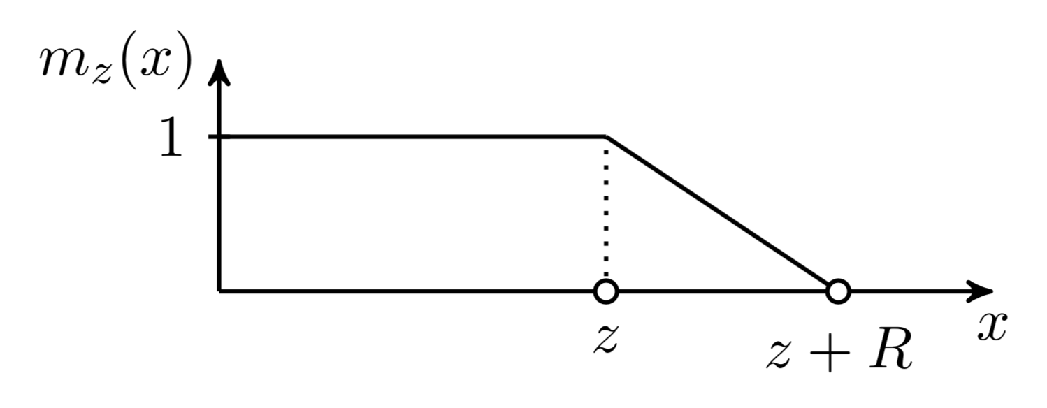
The soft mask function is applied to the softmax elements when computing attention weights:
In the equation above, $z$ is differentiable and is therefore trained jointly with the rest of the model. Parameters $z^{(i)}, i=1, \dots, h$ are learned separately per head. In addition, the loss includes an extra L1 penalty on $\sum_{i=1}^h z^{(i)}$.
Using Adaptive Computation Time, the method can be extended to support a flexible attention span length that adapts dynamically to the current input. The span parameter $z_t$ for an attention head at time $t$ is defined as a sigmoidal function, $z_t = S \sigma(\mathbf{v} \cdot \mathbf{x}_t +b)$, where the vector $\mathbf{v}$ and bias scalar $b$ are learned jointly with other parameters.
In experiments on Transformers with adaptive attention span, Sukhbaatar, et al. (2019) observed a general tendency: lower layers typically do not require long attention spans, while a small number of heads in higher layers may use exceptionally long spans. Adaptive attention span also substantially reduces FLOPS, particularly in large models with many attention layers and long context lengths.
Depth-Adaptive Transformer
At inference time, it is reasonable to assume that some tokens are easier to predict and therefore require less computation than others. Accordingly, a token’s prediction could be processed through only a subset of layers to achieve a better trade-off between speed and performance.
Both Depth-Adaptive Transformer (Elabyad et al. 2020) and Confident Adaptive Language Model (CALM; Schuster et al. 2022) are motivated by this idea, and they learn to predict the optimal number of layers for different input tokens.
Depth-adaptive transformer (Elabyad et al. 2020) attaches an output classifier to every layer, enabling exit predictions based on that layer’s activations. The classifier weight matrices may be distinct per layer or shared across layers. During training, the model samples different sequences of exits so that optimization occurs using hidden states from different layers. The learning objective incorporates likelihood probabilities predicted at different layers, $n=1, \dots, N$:
Adaptive depth classifiers output a parametric distribution $q_t$. Training uses cross-entropy loss against an oracle distribution $q^*_t$. The paper explored three confiurations for learning such a classifier $q_t$.
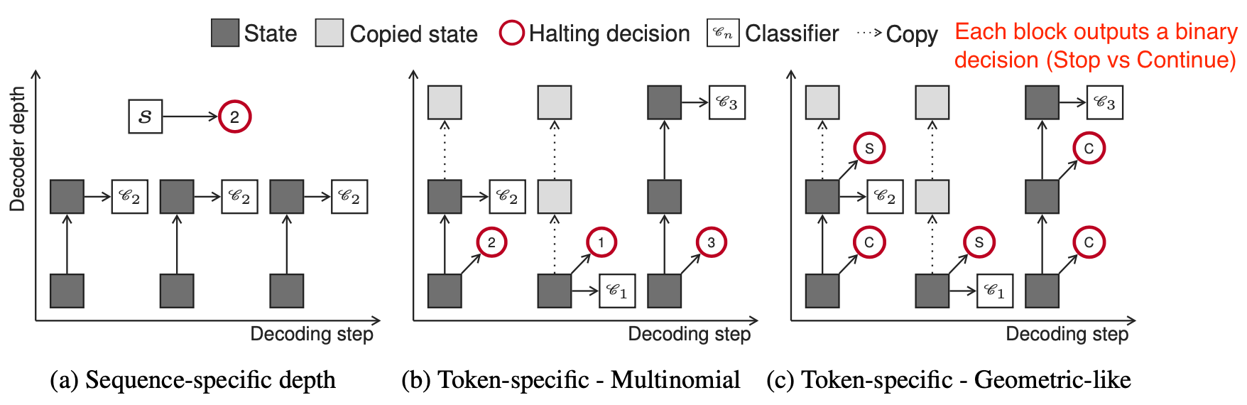
(Image source: Elabyad et al. 2020).
-
Sequence-specific depth classifier: All tokens within the same sequence share a single exit block. The decision depends on the average of the encoder representation for the sequence. Given an input sequence $\mathbf{x}$ of length $L$, the classifier takes $\bar{\mathbf{x}} = \frac{1}{L} \sum_{t=1}^L \mathbf{x}_t$ as input and outputs a multinomial distribution with $N$ dimensions, corresponding to $N$ layers.
$ \begin{aligned} q(n \vert \mathbf{x}) &=\text{softmax}(\mathbf{W}_n \bar{\mathbf{x}} + b_n) \in \mathbb{R}^N \\ q_\text{lik}^*(\mathbf{x}, \mathbf{y}) &= \delta(\arg\max_n \text{LL}^n - \lambda n) \\ \text{or }q_\text{corr}^*(\mathbf{x}, \mathbf{y}) &= \delta(\arg\max_n C^n - \lambda n) \text{ where }C^n = \vert\{t \vert y_t = \arg\max_y p(y \vert \mathbf{h}^n_{t-1})\}\vert \\ \end{aligned} $where $\delta$ is the dirac delta (unit impulse) function, and $-\lambda n$ is a regularization term that encourages exits at lower layers. The ground-truth $q^*$ can be constructed in two ways, based on maximum likelihood $q_\text{lik}^*$ or correctness $q_\text{corr}^*$.
-
Token-specific depth classifier (multinomial): Each token is decoded using a different exit block, predicted conditionally on the first decoder hidden state $\mathbf{h}^1_t$:
$ q_t(n \vert \mathbf{x}, \mathbf{y}_{< t}) = \text{softmax}(\mathbf{W}_n \mathbf{h}^1_t + b_n) $
-
Token-specific depth classifier (geometric-like): A binary exit prediction distribution is produced per layer per token, $\mathcal{X}^n_t$. The RBF kernel $\kappa(t, t’) = \exp(\frac{\vert t - t’ \vert^2}{\sigma})$ is used to smooth predictions, incorporating the impact of the current decision on future time steps.
$ \begin{aligned} \mathcal{X}^n_t &= \text{sigmoid}(\mathbf{w}_n^\top \mathbf{h}^n_t + b_n)\quad \forall n \in [1, \dots, N-1] \\ q_t(n \vert \mathbf{x}, \mathbf{y}_{< t}) &= \begin{cases} \mathcal{X}^n_t \prod_{n' < n} (1 - \mathcal{X}^{n'}_t) & \text{if } n < N\\ \prod_{n' < N} (1 - \mathcal{X}^{n'}_t) & \text{otherwise} \end{cases} \\ q_\text{lik}^*(\mathbf{x}, \mathbf{y}) &= \delta(\arg\max_n \widetilde{\text{LL}}^n_t - \lambda n) \text{ where } \widetilde{\text{LL}}^n_t = \sum_{t'=1}^{\vert\mathbf{y}\vert}\kappa(t, t') LL^n_{t'} \\ \text{or }q_\text{cor}^*(\mathbf{x}, \mathbf{y}) &= \delta(\arg\max_n \tilde{C}_t^n - \lambda n) \text{ where }C_t^n = \mathbb{1}[y_t = \arg\max_y p(y \vert \mathbf{h}^n_{t-1})],\; \tilde{C}^n_t = \sum_{t'=1}^{\vert\mathbf{y}\vert}\kappa(t, t') C^n_{t'} \\ \end{aligned} $
At inference time, the confidence threshold used to decide when to exit must be calibrated. Depth-adaptive transformer identifies this threshold on a validation set via grid search. CALM (Schuster et al. 2022) applied the Learn then Test (LTT) framework (Angelopoulos et al. 2021) to determine a subset of valid thresholds, then selected the minimum value as the inference threshold. In addition to training per-layer exit classifiers, CALM explored other approaches for adaptive depth prediction, including softmax responses (that is, the difference between the top two softmax outputs) and hidden-state saturation (that is, $\cos(\mathbf{h}^n_t, \mathbf{h}^{n+1}_t)$) as confidence scores for exit decisions. They found that softmax responses yielded the best inference speedup.
Efficient Attention
In the vanilla Transformer, computation and memory scale quadratically with sequence length, which makes very long sequences difficult to handle. Many architectural efficiency improvements focus on the self-attention module, aiming to make it cheaper, smaller, or faster. See the survey on Efficient Transformers (Tay et al. 2020).
Sparse Attention Patterns
Fixed Local Context
A straightforward modification for reducing self-attention cost is to restrict each token’s attention span to local context only, so that self-attention scales linearly with sequence length.
This idea was introduced in Image Transformer (Parmer, et al 2018), which frames image generation as sequence modeling using an encoder-decoder Transformer architecture:
- The encoder produces a contextualized, per-pixel-channel representation of the source image.
- The decoder then autoregressively generates an output image, producing one channel per pixel at each time step.
Let the representation of the current pixel to be generated be the query $\mathbf{q}$. The other positions whose representations are used to compute $\mathbf{q}$ are key vectors $\mathbf{k}_1, \mathbf{k}_2, \dots$, and together they form a memory matrix $\mathbf{M}$. The scope of $\mathbf{M}$ specifies the context window for pixel query $\mathbf{q}$.
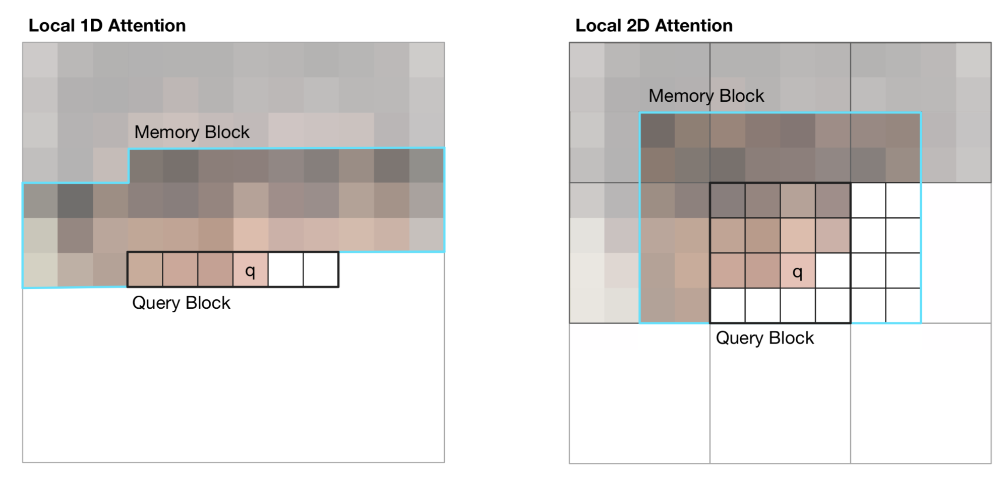
Image Transformer introduced two localized variants of $\mathbf{M}$, as illustrated below.
-
1D Local Attention: The input image is flattened in raster scanning order, from left to right and top to bottom. The linearized image is then partitioned into non-overlapping query blocks. The context window includes pixels in the same query block as $\mathbf{q}$, plus a fixed number of additional pixels generated before that query block.
-
2D Local Attention: The image is partitioned into multiple non-overlapping rectangular query blocks. The query pixel can attend to all other pixels within the same memory blocks. To ensure that the pixel in the top-left corner still has a valid context window, the memory block is extended upward, leftward, and rightward by fixed amounts, respectively.
Strided Context
Sparse Transformer (Child et al., 2019) introduced factorized self-attention via sparse matrix factorization, enabling training of dense attention networks with hundreds of layers on sequences up to length 16,384, which would otherwise be infeasible on modern hardware.
Consider an attention connectivity pattern $\mathcal{S} = \{S_1, \dots, S_n\}$, where each $S_i$ specifies the set of key positions attended to by the $i$-th query vector.
Note that while the size of $S_i$ is not fixed, $a(\mathbf{x}_i, S_i)$ is always of size $d_v$, and thus $\text{Attend}(\mathbf{X}, \mathcal{S}) \in \mathbb{R}^{L \times d_v}$.
In autoregressive models, one attention span is defined as $S_i = \{j: j \leq i\}$, since it allows each token to attend to all past positions.
In factorized self-attention, the set $S_i$ is decomposed into a tree of dependencies such that, for every pair of $(i, j)$ where $j \leq i$, there exists a path connecting $i$ back to $j$, and $i$ can attend to $j$ either directly or indirectly.
More precisely, the set $S_i$ is partitioned into $p$ non-overlapping subsets, where the $m$-th subset is denoted $A^{(m)}_i \subset S_i, m = 1,\dots, p$. As a result, the path between output position $i$ and any $j$ has maximum length $p + 1$. For example, if $(j, a, b, c, \dots, i)$ is a path of indices between $i$ and $j$, then $j \in A_a^{(1)}, a \in A_b^{(2)}, b \in A_c^{(3)}, \dots$, and so forth.
Sparse Factorized Attention
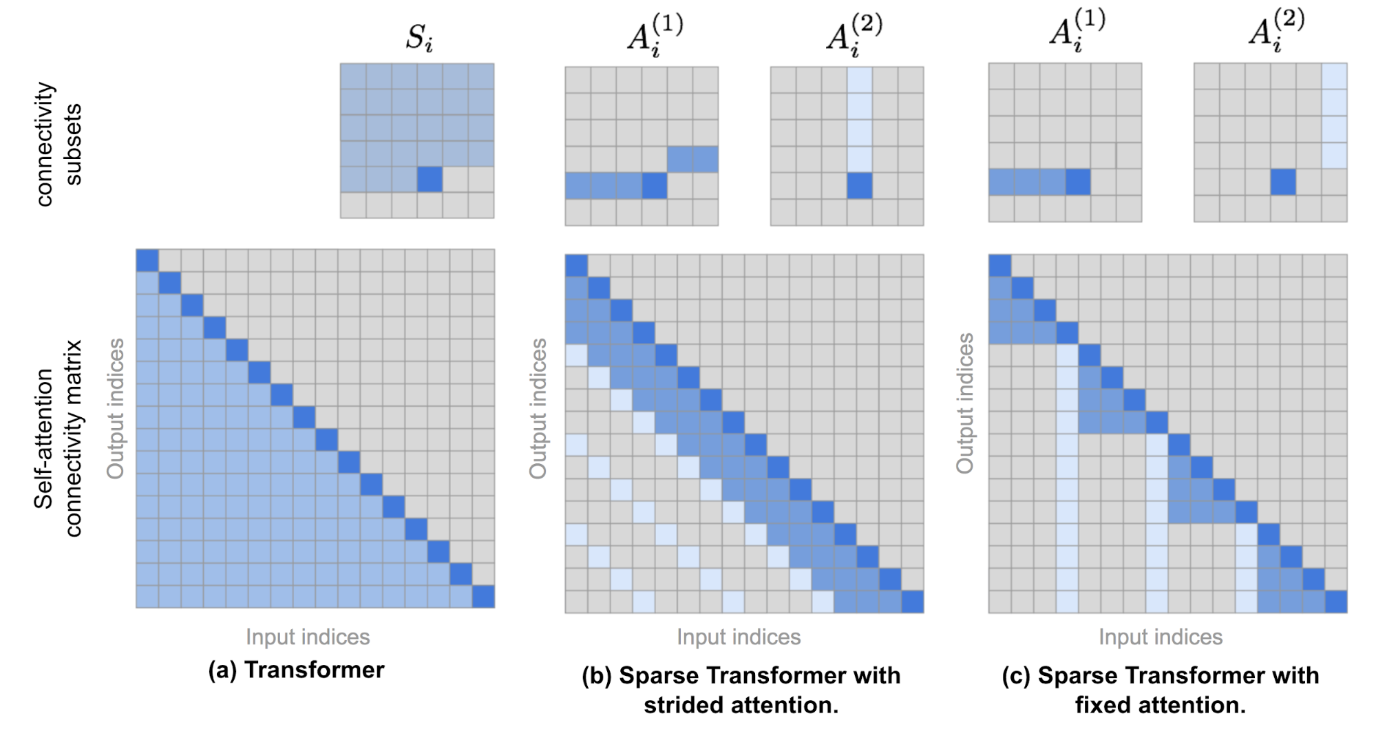
Sparse Transformer proposed two forms of fractorized attention. The concepts are most easily understood using the 2D image examples illustrated in Fig. 10.
-
Strided attention with stride $\ell \sim \sqrt{n}$. This pattern works particularly well for image data because the structure aligns naturally with strides. In the image setting, each pixel attends to all previous $\ell$ pixels in raster-scan order (thereby covering the full width of the image), and those pixels then attend to others in the same column (as defined by another attention-connectivity subset).
$ \begin{aligned} A_i^{(1)} &= \{ t, t+1, \dots, i\} \text{, where } t = \max(0, i - \ell) \\ A_i^{(2)} &= \{j: (i-j) \mod \ell = 0\} \end{aligned} $
-
Fixed attention. A small set of tokens summarizes prior locations and propagates that information to all subsequent locations.
$ \begin{aligned} A_i^{(1)} &= \{j: \lfloor \frac{j}{\ell} \rfloor = \lfloor \frac{i}{\ell} \rfloor \} \\ A_i^{(2)} &= \{j: j \mod \ell \in \{\ell-c, \dots, \ell-1\} \} \end{aligned} $where $c$ is a hyperparameter. If $c=1$, the representation becomes constrained because many positions depend on only a few locations. The paper selected $c\in \{ 8, 16, 32 \}$ for $\ell \in \{ 128, 256 \}$.
Use Factorized Self-Attention in Transformer
There are three approaches for incorporating sparse, factorized attention patterns into the Transformer architecture:
- Assign one attention type per residual block and interleave them,
$\text{attn}(\mathbf{X}) = \text{Attend}(\mathbf{X}, A^{(n \mod p)}) \mathbf{W}^o$, where $n$ denotes the index of the current residual block. - Introduce a single head that attends to the union of locations attended by all factorized heads,
$\text{attn}(\mathbf{X}) = \text{Attend}(\mathbf{X}, \cup_{m=1}^p A^{(m)}) \mathbf{W}^o $. - Use multi-head attention, but unlike the vanilla Transformer, each head may adopt one of the patterns described above (1 or 2). $\rightarrow$ This option often yields the best performance.
Sparse Transformer also proposed a set of modifications to enable training Transformers with hundreds of layers, including gradient checkpointing, recomputing attention and FF layers during the backward pass, mixed precision training, efficient block-sparse implementations, and more. For additional details, see the paper or my earlier post on techniques for scaling up model training.
Blockwise Attention (Qiu et al. 2019) introduces a sparse block matrix that limits each token to attending to only a small subset of other tokens. Each attention matrix of size $L \times L$ is partitioned into $n \times n$ smaller blocks of size $\frac{L}{n}\times\frac{L}{n}$, and a sparse block matrix $\mathbf{M} \in \{0, 1\}^{L \times L}$ is defined by a permutation $\pi$ of ${1, \dots, n}$, which records the column index for each row in the block matrix.
In practice, Blockwise Attention stores QKV only as block matrices, each of size $n\times n$:
where $\hat{\mathbf{q}}_i$, $\hat{\mathbf{k}}_i$, and $\hat{\mathbf{v}}_i$ are the $i$-th row in the QKV block matrix, respectively. Each $\mathbf{q}_i\mathbf{k}_{\pi(i)}^\top, \forall i = 1, \dots, n$ has size $\frac{N}{n}\times\frac{N}{n}$, and therefore Blockwise Attention can reduce the attention-matrix memory complexity from $\mathcal{O}(L^2)$ to $\mathcal{O}(\frac{L}{n}\times\frac{L}{n} \times n) = \mathcal{O}(L^2/n)$.
Combination of Local and Global Context
ETC (Extended Transformer Construction; Ainslie et al. 2019), Longformer (Beltagy et al. 2020), and Big Bird (Zaheer et al. 2020) combine local and global context when constructing the attention matrix. All of these models can be initialized from existing pretrained models.
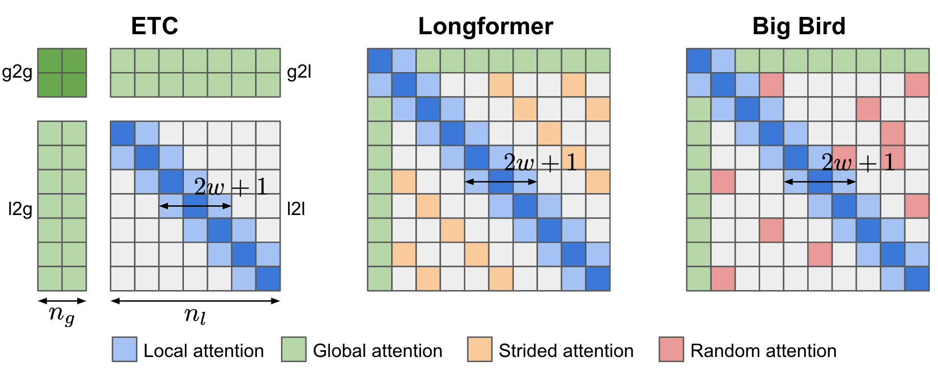
Global-Local Attention in ETC (Ainslie et al. 2019) takes two inputs: (1) the long input $\mathbf{x}^l$ of size $n_l$, which is the standard input sequence; and (2) the global input $\mathbf{x}^g$ of size $n_g$, which contains a smaller set of auxiliary tokens, $n_g \ll n_l$. Attention is then divided into four components, based on directional attention between the two inputs: g2g, g2l, l2g, and l2l. Because the l2l component can be very large, it is constrained to a fixed attention span with radius $w$ (that is, a local attention span), and the l2l matrix can be reshaped to $n_l \times (2w+1)$.
ETC uses four binary matrices to support structured inputs, $\mathbf{M}^{g2g}$, $\mathbf{M}^{g2l}$, $\mathbf{M}^{l2g}$, and $\mathbf{M}^{l2l}$. For example, each element $z^g_i \in \mathbb{R}^d$ in the attention output $z^g = (z^g_1, \dots, z^g_{n_g})$ for the g2g attention component is defined as:
where $P^K_{ij}$ is a learnable vector for relative position encoding, and $C$ is a very large constant ($C=10000$ in the paper) used to offset attention weights when the mask is off.
ETC also adds a CPC (contrastive predictive coding) objective during pretraining, using NCE loss, in addition to the MLM task: the representation of a sentence should be similar to the representation of its surrounding context when that sentence is masked.
The global input $\mathbf{x}^g$ for ETC is constructed as follows. Assuming the long input contains segments (for example, by sentence), each segment is paired with one auxiliary token to learn global inputs. Relative position encoding is used to annotate global segment tokens with the token position. Hard masking in one direction (that is, labeling tokens before versus after differently) was found to improve performance on some datasets.
The Longformer attention pattern consists of three components:
- Local attention: As in ETC, local attention is controlled via a sliding window of fixed size $w$;
- Global attention for preselected tokens: Longformer designates a small number of preselected tokens (for example, the
[CLS]token) to have global attention span, meaning they attend to all other tokens in the input sequence. - Dilated attention: A dilated sliding window of fixed size $r$ with gaps of dilation size $d$, similar to Sparse Transformer;
Big Bird is broadly similar to Longformer: it uses local attention and a small set of preselected tokens with global attention span. However, Big Bird replaces dilated attention with a new mechanism in which all tokens attend to a set of random tokens. This design is motivated by viewing the attention pattern as a directed graph; a random graph has the property that information can propagate quickly between any pair of nodes.
Longformer uses smaller window sizes in lower layers and larger window sizes in higher layers. Ablation studies showed that this configuration outperforms the reversed or fixed-size alternatives. Lower layers omit dilated sliding windows to better learn how to use immediate local context. Longformer also uses a staged training procedure: the model is first trained with a small window size to learn from local context; later stages increase window sizes and decrease the learning rate.
Content-based Attention
The improvements introduced by Reformer (Kitaev, et al. 2020) target the following pain points in the vanilla Transformer:
- Quadratic time and memory complexity in the self-attention module.
- In a model with $N$ layers, memory is $N$-times larger than in a single-layer model because activations must be stored for back-propagation.
- The intermediate FF layers are often quite large.
Reformer introduces two primary changes:
- It replaces dot-product attention with locality-sensitive hashing (LSH) attention, reducing complexity from $\mathcal{O}(L^2)$ to $\mathcal{O}(L\log L)$.
- It replaces standard residual blocks with reversible residual layers, enabling activations to be stored only once during training rather than $N$ times (that is, proportional to the number of layers).
Locality-Sensitive Hashing Attention
In the $\mathbf{Q} \mathbf{K}^\top$ part of the attention formula, we care primarily about the largest elements, since only large values contribute meaningfully after softmax. For each query $\mathbf{q}_i \in \mathbf{Q}$, we want to find the row vectors in $\mathbf{K}$ that are closest to $\mathbf{q}_i$. To find nearest neighbors efficiently in high-dimensional space, Reformer integrates Locality-Sensitive Hashing (LSH) into the attention mechanism.
A hashing scheme $x \mapsto h(x)$ is locality-sensitive if it preserves distance information between data points, such that nearby vectors receive similar hashes while distant vectors receive very different hashes. Reformer adopts such a hashing scheme. Given a fixed random matrix $\mathbf{R} \in \mathbb{R}^{d \times b/2}$ (where $b$ is a hyperparameter), the hash function is $h(x) = \arg\max([xR; −xR])$.
If we drop the scalar in self-attention and condense the denominator into a normalizing term $Z(.)$, a standard attention output can be written as follows: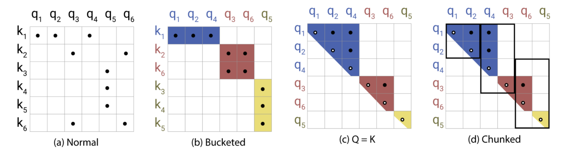
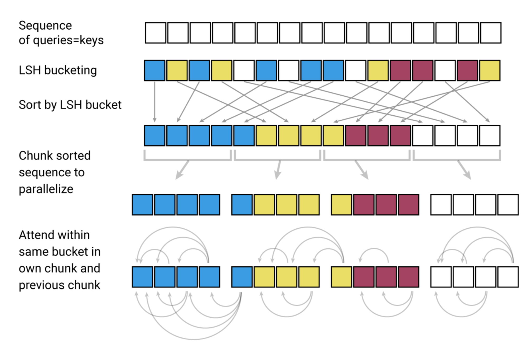
With LSH attention, a query may attend only to positions within the same hashing bucket, $S_i = \{j: h(\mathbf{q}_i) = h(\mathbf{k}_j)\}$. The procedure is as follows (illustrated in Fig. 20):
- (a) The full-attention matrix is often sparse.
- (b) With LSH, keys and queries can be sorted and aligned according to hash buckets.
- (c) Set $\mathbf{Q} = \mathbf{K}$ (specifically $\mathbf{k}_j = \mathbf{q}_j / |\mathbf{q}_j|$) so that each bucket contains equal numbers of keys and queries, which simplifies batching. Notably, this “shared-QK” configuration does not affect Transformer performance.
- (d) Apply batching by grouping chunks of $m$ consecutive queries.
Reversible Residual Network
Another Reformer improvement is the use of reversible residual layers (Gomez et al. 2017). The goal of a reversible residual network is to design layers such that the activations at any layer can be reconstructed from the activations at the subsequent layer using only model parameters. This enables memory savings by recomputing activations during backpropagation, rather than storing all intermediate activations.
Given a layer $x \mapsto y$, a standard residual layer performs $y = x + F(x)$. In contrast, a reversible layer splits both input and output into pairs $(x_1, x_2) \mapsto (y_1, y_2)$ and then applies:
Reversing the transformation is straightforward:
Reformer applies this concept to Transformers by combining attention ($F$) and feed-forward layers ($G$) within a reversible network block:
Memory usage can be reduced even further by chunking the feed-forward computation:
With this construction, the reversible Transformer does not need to store activations at every layer.
Routing Transformer (Roy et al. 2021) also relies on content-based clustering of keys and queries. Rather than using a static hashing function like LSH, it applies online $k$-means clustering and combines it with local, temporal sparse attention to reduce attention complexity from $O(L^2)$ to $O(L^{1.5})$.
In routing attention, both keys and queries are clustered using the $k$-means method, sharing the same set of centroids $\boldsymbol{\mu} = (\mu_1, \dots, \mu_k) \in \mathbb{R}^{k \times d}$. Queries are routed to keys assigned to the same centroid. Total complexity is $O(Lkd + L^2d/k)$, where $O(Lkd)$ accounts for clustering assignments and $O(L^2d/k)$ accounts for attention computation. Cluster centroids are updated via EMA (exponential moving average) using all associated keys and queries.
In Routing Transformer experiments, some of the best configurations enable routing attention only in the final two layers and for half of the attention heads, while the remaining heads use local attention. The authors also observed that local attention is a strong baseline, and that larger attention windows consistently produce better results.
Low-Rank Attention
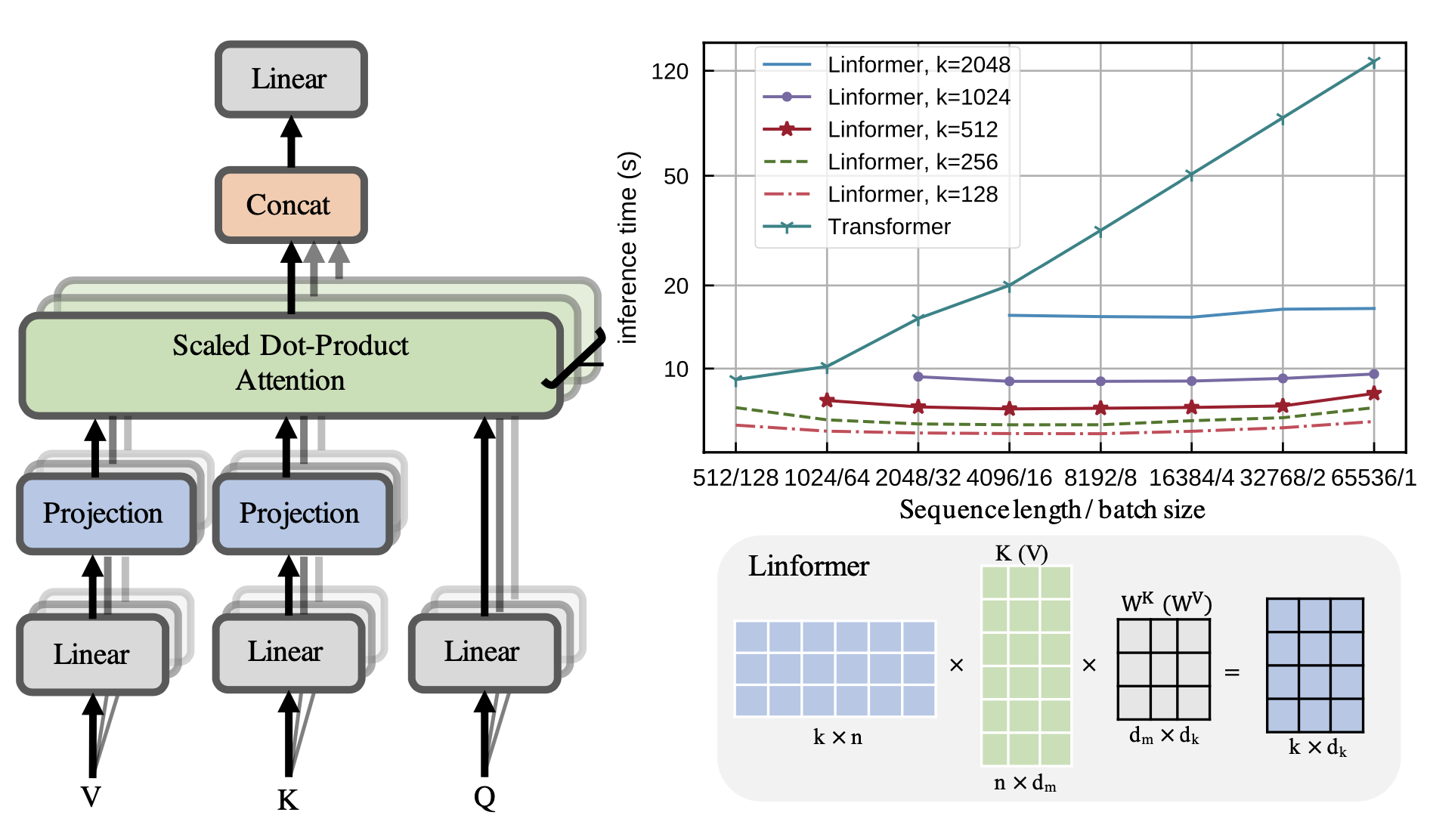
Linformer (Wang et al. 2020) approximates the full attention matrix with a low-rank matrix, reducing time and space complexity to linear. Rather than using an expensive SVD to find a low-rank decomposition, Linformer introduces two linear projections $\mathbf{E}_i, \mathbf{F}_i \in \mathbb{R}^{L \times k}$ for the key and value matrices, respectively, reducing their dimensions from $L \times d$ to $k \times d$. As long as $k \ll L$, attention memory can be reduced substantially.
Additional techniques can further improve Linformer efficiency:
- Share parameters between projection layers, including head-wise, key-value, and layer-wise (across all layers) sharing.
- Use different $k$ at different layers. Because heads in higher layers tend to exhibit a more skewed distribution (lower rank), a smaller $k$ can be used in higher layers.
- Use alternative projection types, such as mean or max pooling, or a convolution layer with kernel and stride $L/k$.
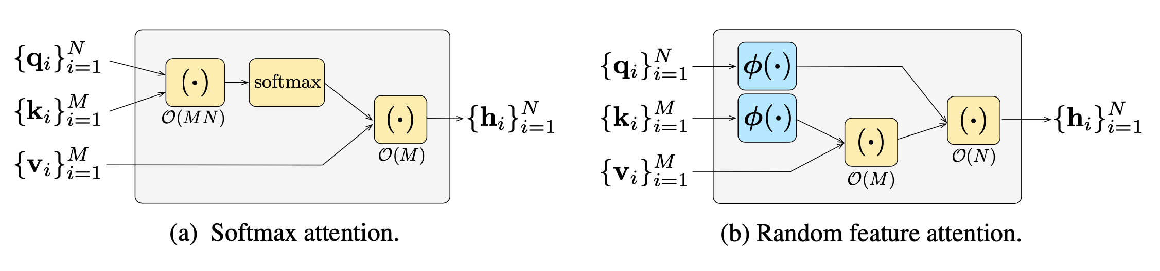
Random Feature Attention (RFA; Peng et al. 2021) uses random feature methods (Rahimi & Recht, 2007) to approximate the softmax in self-attention via low-rank feature maps, achieving linear time and space complexity. Performers (Choromanski et al. 2021) also adopts random feature attention, improving kernel construction to further reduce kernel approximation error.
The main theorem behind RFA is from Rahimi & Recht, 2007:
Let $\phi: \mathbb{R}^d \to \mathbb{R}^{2D}$ be a nonlinear transformation:
$ \phi(\mathbf{x}) = \frac{1}{\sqrt{D}}[\sin(\mathbf{w}_1^\top \mathbf{x}), \dots, \sin(\mathbf{w}_D^\top \mathbf{x}), \cos(\mathbf{w}_1^\top \mathbf{x}), \dots, \cos(\mathbf{w}_D^\top \mathbf{x})]^\top $When $d$-dimensional random vectors $\mathbf{w}_i$ are i.i.d. from $\mathcal{N}(\mathbf{0}, \sigma^2\mathbf{I}_d)$, $ \mathbb{E}_{\mathbf{w}_i} [\phi(\mathbf{x}) \cdot \phi(\mathbf{y})] = \exp(-\frac{\| \mathbf{x} - \mathbf{y} \|^2}{2\sigma^2}) $
An unbiased estimate of $\exp(\mathbf{x} \cdot \mathbf{y})$ is:
We can then express the attention function as follows, where $\otimes$ is the outer product operation and $\sigma^2$ is the temperature:
Causal Attention RFA has each token at time step $t$ attend only to earlier keys and values $\{\mathbf{k}_i\}_{i \leq t}, \{\mathbf{v}_i\}_{i \leq t}$. To track hidden-state history at time step $t$, similarly to RNNs, we use a tuple of variables $(\mathbf{S}_t \in \mathbb{R}^{2D \times d}, \mathbf{z} \in \mathbb{R}^{2D})$:
where $2D$ is the size of $\phi(.)$, and $D$ should be no less than the model size $d$ for a reasonable approximation.
RFA leads to significant speedups in autoregressive decoding, and its memory complexity depends mainly on the choice of $D$ when constructing the kernel $\phi(.)$.
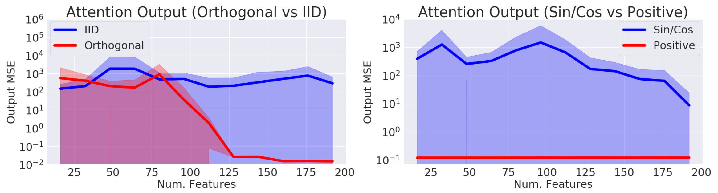
Performer modifies random feature attention by using positive random feature maps to reduce estimation error. It also constrains the randomly sampled $\mathbf{w}_1, \dots, \mathbf{w}_D$ to be orthogonal, further reducing estimator variance.
Transformers for Reinforcement Learning
Self-attention avoids compressing the entire past into a fixed-size hidden state, and it is less prone to vanishing or exploding gradients than RNNs. Reinforcement learning tasks can certainly benefit from these properties. However, training Transformers can be difficult even in supervised settings, and it is even more challenging in the RL context. After all, stabilizing and training an LSTM agent alone can already be quite hard.
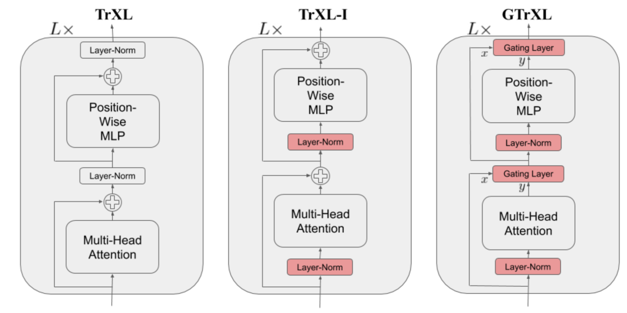
Gated Transformer-XL (GTrXL; Parisotto, et al. 2019) is one attempt to apply Transformers to RL. Building on Transformer-XL, GTrXL stabilized training through two changes:
- Layer normalization is applied only to the input stream within a residual module, and not to the shortcut stream. A key advantage of this reordering is that it allows the original input to propagate from the first layer to the last.
- The residual connection is replaced by a GRU-style (Gated Recurrent Unit; Chung et al., 2014) gating mechanism.
The gating-function parameters are explicitly initialized to be close to an identity map, which is why the $b_g$ term appears. A $b_g > 0$ greatly improves learning speed.
Decision Transformer (DT; Chen et al 2021) casts reinforcement learning as conditional sequence modeling, producing optimal actions conditioned on the desired return, as well as past states and actions. This formulation makes it straightforward to use a Transformer architecture. Decision Transformer targets off-policy RL, where the model has access only to a fixed set of trajectories collected by other policies.
To encourage the model to learn actions that achieve a desired return, DT feeds the model the desired future return $\hat{R} = \sum_{t’=t}^T r_{t’}$ rather than the current reward. The trajectory is represented as a list of triplets, (return-to-go $\hat{R}_t, state $s_t$, action $a_t$), and this list is used as the input sequence to the Transformer:
Three linear layers are added and trained, one each for return-to-go, state, and action, to produce token embeddings. The prediction head is trained to predict $a_t$ corresponding to the input token $s_t$. Training uses cross-entropy loss for discrete actions or MSE for continuous actions. In their experiments, predicting states or return-to-go did not improve performance.
Experiments compared DT with several model-free RL algorithm baselines and showed that:
- DT is more efficient than behavior cloning in low-data regimes;
- DT models the distribution of returns effectively;
- Long context is crucial for strong performance;
- DT can handle sparse rewards.
Citation
Cited as:
Weng, Lilian. (Jan 2023). The transformer family version 2.0. Lil’Log. https://lilianweng.github.io/posts/2023-01-27-the-transformer-family-v2/.
Or
@article{weng2023transformer,
  title   = "The Transformer Family Version 2.0",
  author  = "Weng, Lilian",
  journal = "lilianweng.github.io",
  year    = "2023",
  month   = "Jan",
  url     = "https://lilianweng.github.io/posts/2023-01-27-the-transformer-family-v2/"
}
References
[1] Ashish Vaswani, et al. “Attention is all you need.” NIPS 2017.
[2] Rami Al-Rfou, et al. “Character-level language modeling with deeper self-attention.” AAAI 2019.
[3] Olah & Carter, “Attention and Augmented Recurrent Neural Networks”, Distill, 2016.
[4] Sainbayar Sukhbaatar, et al. “Adaptive Attention Span in Transformers”. ACL 2019.
[5] Rewon Child, et al. “Generating Long Sequences with Sparse Transformers” arXiv:1904.10509 (2019).
[6] Nikita Kitaev, et al. “Reformer: The Efficient Transformer” ICLR 2020.
[7] Alex Graves. (“Adaptive Computation Time for Recurrent Neural Networks”)[https://arxiv.org/abs/1603.08983]
[8] Niki Parmar, et al. “Image Transformer” ICML 2018.
[9] Zihang Dai, et al. “Transformer-XL: Attentive Language Models Beyond a Fixed-Length Context.” ACL 2019.
[10] Aidan N. Gomez, et al. “The Reversible Residual Network: Backpropagation Without Storing Activations” NIPS 2017.
[11] Mostafa Dehghani, et al. “Universal Transformers” ICLR 2019.
[12] Emilio Parisotto, et al. “Stabilizing Transformers for Reinforcement Learning” arXiv:1910.06764 (2019).
[13] Rae et al. “Compressive Transformers for Long-Range Sequence Modelling.” 2019.
[14] Press et al. “Train Short, Test Long: Attention With Linear Biases Enables Input Length Extrapolation.” ICLR 2022.
[15] Wu, et al. “DA-Transformer: Distance Aware Transformer” 2021.
[16] Elabyad et al. “Depth-Adaptive Transformer.” ICLR 2020.
[17] Schuster et al. “Confident Adaptive Language Modeling” 2022.
[18] Qiu et al. “Blockwise self-attention for long document understanding” 2019.
[19] Roy et al. “Efficient Content-Based Sparse Attention with Routing Transformers.” 2021.
[20] Ainslie et al. “ETC: Encoding Long and Structured Inputs in Transformers.” EMNLP 2019.
[21] Beltagy et al. “Longformer: The long-document transformer.” 2020.
[22] Zaheer et al. “Big Bird: Transformers for Longer Sequences.” 2020.
[23] Wang et al. “Linformer: Self-Attention with Linear Complexity.” arXiv preprint arXiv:2006.04768 (2020).
[24] Tay et al. 2020 “Sparse Sinkhorn Attention.” ICML 2020.
[25] Peng et al. “Random Feature Attention.” ICLR 2021.
[26] Choromanski et al. “Rethinking Attention with Performers.” ICLR 2021.
[27] Khandelwal et al. “Generalization through memorization: Nearest neighbor language models.” ICLR 2020.
[28] Yogatama et al. “Adaptive semiparametric language models.” ACL 2021.
[29] Wu et al. “Memorizing Transformers.” ICLR 2022.
[30] Su et al. “Roformer: Enhanced transformer with rotary position embedding.” arXiv preprint arXiv:2104.09864 (2021).
[31] Shaw et al. “Self-attention with relative position representations.” arXiv preprint arXiv:1803.02155 (2018).
[32] Tay et al. “Efficient Transformers: A Survey.” ACM Computing Surveys 55.6 (2022): 1-28.
[33] Chen et al., “Decision Transformer: Reinforcement Learning via Sequence Modeling” arXiv preprint arXiv:2106.01345 (2021).