Thinking about High-Quality Human Data
[Special thanks to Ian Kivlichan for many helpful pointers (e.g., the 100+ year old Nature paper “Vox populi”) and for thoughtful feedback. 🙏 ] High-quality data is the fuel that powers training for modern deep learning models. Most task-specific labeled datasets are produced through human annotation, whether for classification tasks or for RLHF labeling (which can be represented in a classification format) used to train LLM alignment. Although many ML techniques discussed in this post can improve data quality, human data collection ultimately depends on close attention to detail and careful execution. The community recognizes the importance of high-quality data, yet there remains a subtle perception that “Everyone wants to do the model work, not the data work” (Sambasivan et al. 2021).
· 20 min read · Curated and presented by Arthur Sedek
[Special thank you to Ian Kivlichan for many helpful pointers (e.g., the 100+ year old Nature paper “Vox populi”) and thoughtful feedback. 🙏 ]
High-quality data is the essential fuel for training modern deep learning models. Most task-specific labeled data is produced through human annotation, such as labels for classification tasks or RLHF labeling (which can be represented in a classification format) for LLM alignment training. Many of the ML techniques covered in this post can improve data quality, but at its core, human data collection depends on careful execution and close attention to detail. The community broadly recognizes the value of high-quality data, yet there remains a subtle perception that “Everyone wants to do the model work, not the data work” (Sambasivan et al. 2021).
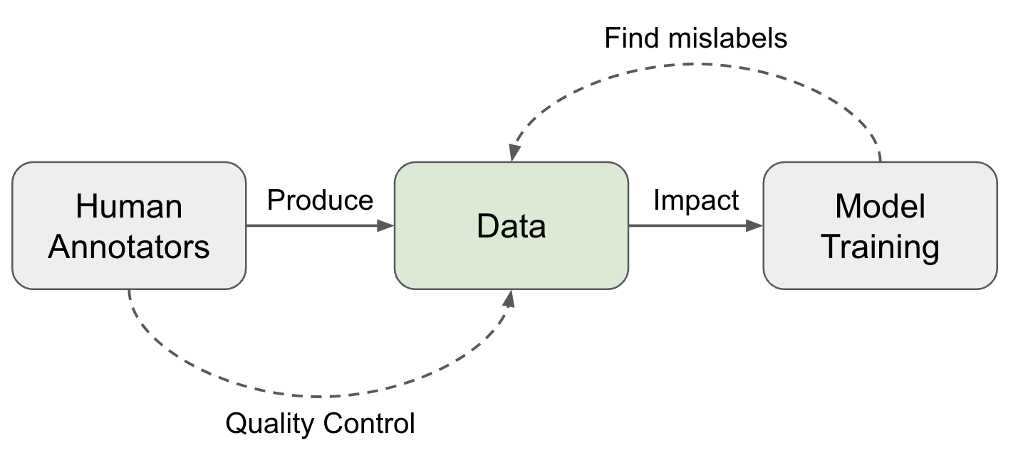
Human Raters ↔ Data Quality
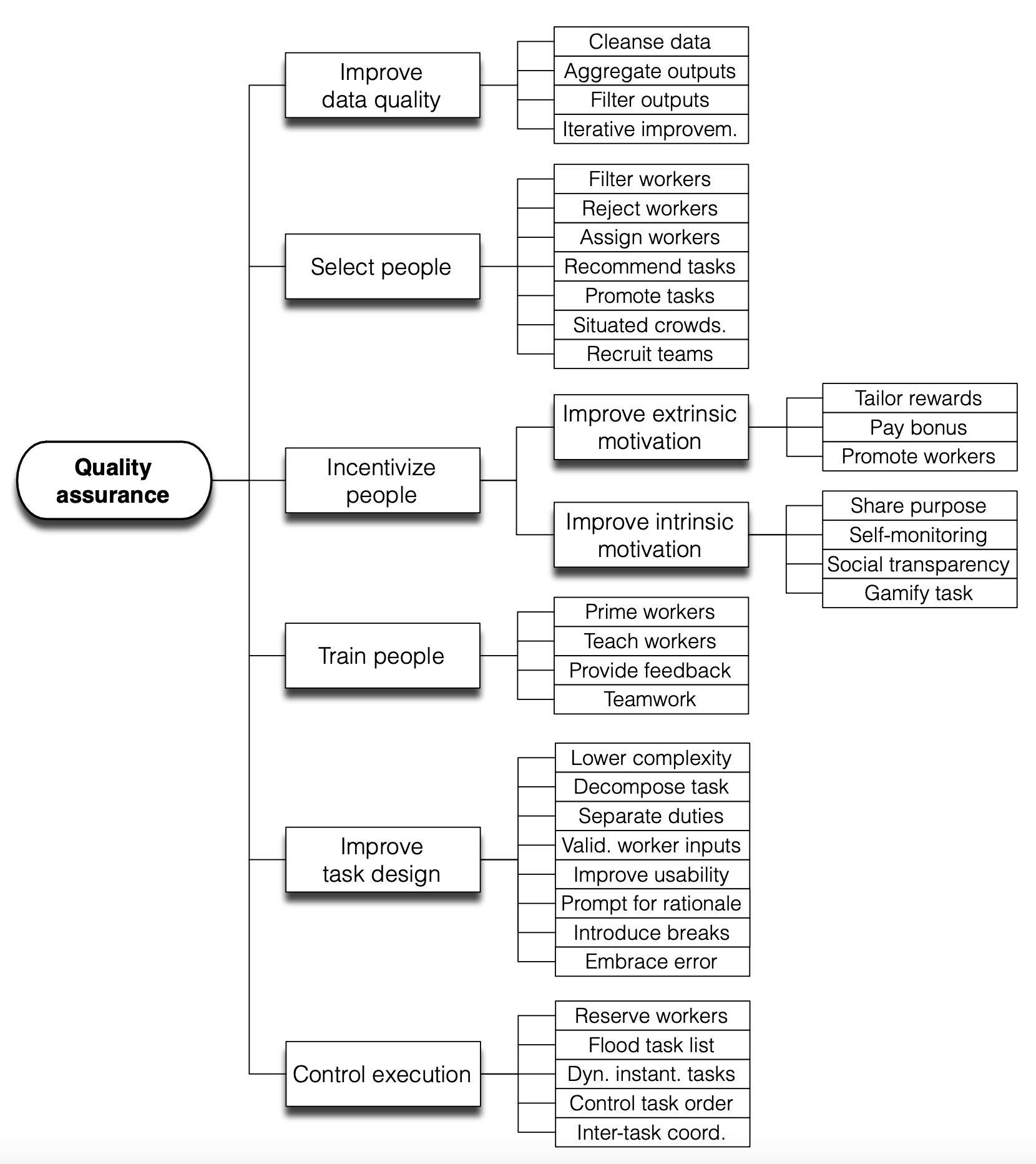
Collecting human-generated data typically involves a sequence of operational steps, and each step affects the resulting data quality:
- Task design: Design the task workflow to increase clarity and reduce complexity. Detailed guidelines can be useful, but overly long or complicated guidelines require substantial training before they become effective.
- Select and train a pool of raters: Choose annotators whose skills align with the task and who demonstrate consistency. Training sessions are necessary. After onboarding, ongoing feedback and periodic calibration sessions are also required.
- Collect and aggregate data: At this stage, additional ML techniques can be applied to clean, filter, and intelligently aggregate the data in order to infer the true labels.
The Wisdom of the Crowd
Vox populi (originally “Vox populi, vox Dei”) is a Latin phrase meaning “the voice of the people.” A short paper with the same name was published in Nature in 1907. It described an event at an annual exhibition in which a fat ox was presented, and attendees were invited to guess the ox’s weight, with a prize awarded for guesses close to the true value. The middlemost estimate was treated as “the vox populi,” and it turned out to be very close to the actual weight. The author concluded: “This result is, I think, more creditable to the trustworthiness of a democratic judgment than might have been expected.” This is likely one of the earliest accounts of how crowdsourcing (the “wisdom of the crowd”) can succeed.
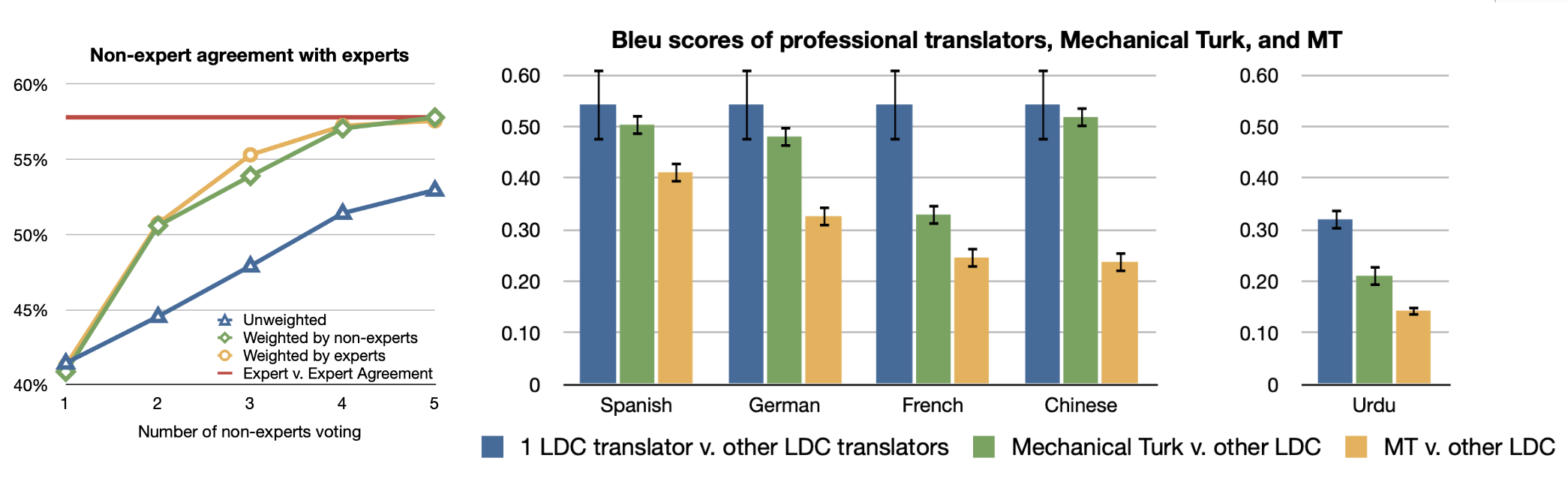
Nearly 100 years later, Callison-Burch (2009) conducted an early study using Amazon Mechanical Turk (AMT) to run non-expert human evaluation for Machine Translation (MT) and even to rely on non-experts to create new gold reference translations. The evaluation task was straightforward: each turker was shown a source sentence, a reference translation, and five translations produced by five MT systems. Turkers were asked to rank the five system outputs from best to worst. Each task was completed by five turkers.
As expected, some spammers produced low-quality annotations while optimizing for volume. Therefore, when measuring agreement between experts and non-experts, Callison-Burch applied weighting schemes that reduce spammers’ impact: (1) “weighted by experts,” which uses each turker’s agreement rate with experts on a gold set of 10 examples; (2) “weighted by non-experts,” which uses each turker’s agreement rate with the remaining turkers across the full dataset.
For a more challenging task, non-expert annotators were asked to produce new gold reference translations. Callison-Burch designed a two-stage process: first, turkers created new translations with reference to MT outputs; second, the process filtered translations that appeared to be generated by an MT system. The correlation between expert translations and crowdsourced translations was higher than the correlation between expert translations and MT system outputs.
Rater Agreement
Annotation is often treated as the process of recovering a single ground truth, and quality is evaluated against one gold answer under consistent standards. A common approach for obtaining reliable ground truth labels is to collect multiple labels from multiple raters. If we assume that raters vary in quality, we can aggregate annotations using a weighted average, where the weights are derived from a proficiency score. In practice, this proficiency score is often approximated by how frequently a rater agrees with others.
Majority Voting: Majority vote is the simplest aggregation method, and it is equivalent to taking the mode of the label set. Under this approach, all annotators contribute equally.
Raw agreement (Tratz & Hovy, 2010): Raw agreement is computed as the percentage of other annotators who agree with a given annotator. This measure is indirectly related to majority voting because annotators who assign the majority label are expected to have higher inter-annotator agreement.
Cohen’s Kappa (Landis & Koch, 1977): Cohen’s kappa measures inter-rater agreement using $\kappa = (p_o - p_e) / (1 - p_c)$, where $p_o$ is the raw agreement rate and $p_e$ is the agreement expected by chance. Cohen’s kappa corrects for chance agreement, but this correction can be overestimated when one label is especially prevalent.
Probabilistic Graph Modeling: A substantial line of work uses probabilistic graph modeling to represent factors that affect annotation decisions, for example, task difficulty, latent topics, rater bias, and rater confidence, and then infer the true labels. Zheng et al. (2017) compared 17 algorithms for truth inference in crowdsourcing, and most were probabilistic graph models.
- MACE (Multi-Annotator Competence Estimation; Hovy et al. 2013) is an early example of using graph modeling to estimate the likelihood that an annotator behaves like a “spammer” by providing random labels. When incentives are misaligned, some annotators may act as spammers to maximize completed task volume for higher pay. MACE aims to identify such spammers. Given a task $i$ and an annotator $j$, $T_i$ is the true label, $A_{ij}$ is the assigned label, and $S_{ij}$ models the probability of annotator $j$ spamming. The generative process can be represented as belows. The parameter $\theta_j$ defines the trustworthiness of the annotator $j$ (probability of not spamming), and the parameter $\xi_j$ defines how an annotator behaves when they are spamming.
We can then learn $\theta, \xi$ by maximizing the observed data via the marginal data likelihood, where $A$ is the matrix of annotations, $S$ is the matrix of competence indicators, and $T$ is the matrix of true labels:
Either EM (Expectation–maximization) or VB (Variational Bayes) can be used to maximize the marginal likelihood above. In EM optimization, during the M-step, a fixed value $\delta$ is added to the fractional counts before normalization. In VB training, symmetric Beta priors are applied to $\theta_j$ and symmetric Dirichlet priors are applied to $\xi_j$. To recover the correct answers, we can take a majority vote weighted by annotators’ $\theta$ estimates.
Rater Disagreement & Two Paradigms
The aggregation approaches above rely on the assumption that there is one underlying gold answer, which makes it possible to evaluate annotator performance accordingly. In many domains, however, especially safety-related, social, or cultural topics, disagreement can be both common and legitimate. In those cases, the key question becomes how strongly we want to enforce a single strict rule versus how much we want to preserve diversity of perspective.
Aroyo & Welty (2015) examined several “myths” in common annotation practice and argued that each is at least somewhat inaccurate. Their key findings include:
- For some samples, more than one interpretation can be correct. Capturing diverse perspectives is important, for example, by having multiple people review annotation quality.
- Disagreement is not inherently negative. Disagreements caused by errors or poor process design should be reduced, but other forms of disagreement can provide valuable information.
- When disagreement stems from an ill-defined task, instructions should be improved. However, more detailed guidelines do not eliminate inherent diversity in opinions.
- Experts are not always better than laypeople, although they may differ substantially in terms of what they consider important.
- Ground truth annotations can shift over time, particularly for timely events or news-related content.
Later, Rottger et al. (2021) articulated this distinction as two contrasting paradigms for annotating subjective NLP tasks.
| Descriptive | Prescriptive | |
|---|---|---|
| Definition | Encourage annotator subjectivity, trying to model many beliefs. | Discourage annotator subjectivity, trying to consistently apply one belief. |
| Pros | - Can help to identify which entries are more subjective; - Embrace diversity |
- More aligned with standard NLP setup. - Easier to do QC by measuring disagreement or doing label aggregation. |
| Cons | - Metrics like rater disagreement cannot be used to measure data quality or annotator performance; - Cannot be used for training models that are optimized for outputting one preset behavior. |
- Expensive and challenging to create high-quality annotation guidelines, which can never be perfect, in practice; - Training annotators to get familiar with guideline in order to apply it properly is also challenging; - Cannot capture an interpretable diversity of beliefs or consistently encode one specific belief. |
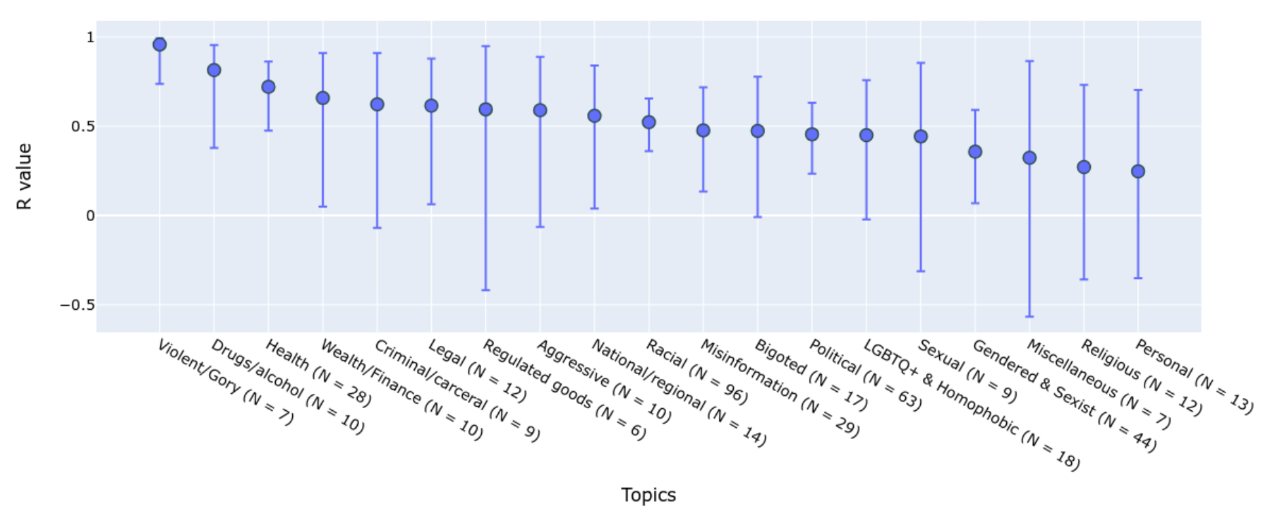
The descriptive paradigm makes it possible to account for different perspectives and to analyze several important effects. For example, annotator identity (e.g., African American, LGBTQ) is a statistically significant factor in whether identity-related content is labeled as toxic (Goyal et al. 2022). Topic is another major driver of divergent views. Wang et al. (2023) studied human evaluation for the safety of an AI conversation system and compared labels from Trust & Safety (T&S) professionals with labels from crowdsourcing annotators. They intentionally collected rich metadata about crowd annotators, such as demographic or behavioral information. When comparing T&S expert labels with crowd annotations, they found that agreement varies substantially by semantic topic and severity level:
- Agreement rates differ greatly across topics, ranging from 0.96 on violence/gory to 0.25 on personal topics.
- Agreement rates are higher for “extreme” and “benign” conversations, given four label options: “benign,” “debatable,” “moderate,” and “extreme.”
Zhang et al. (2023) proposed a taxonomy of rater disagreement to analyze underlying causes. Among the causes they identify, disagreement resulting from stochastic errors or individual-level inconsistency should be minimized. When a rater assigns different labels to the same task across repeated presentations, at least some cases are likely attributable to human error. Motivated by this, the disagreement deconvolution method (Gordon et al. 2021) separates stable opinions from errors by anchoring each individual’s opinion to their own primary label, thereby encouraging intra-rater consistency.
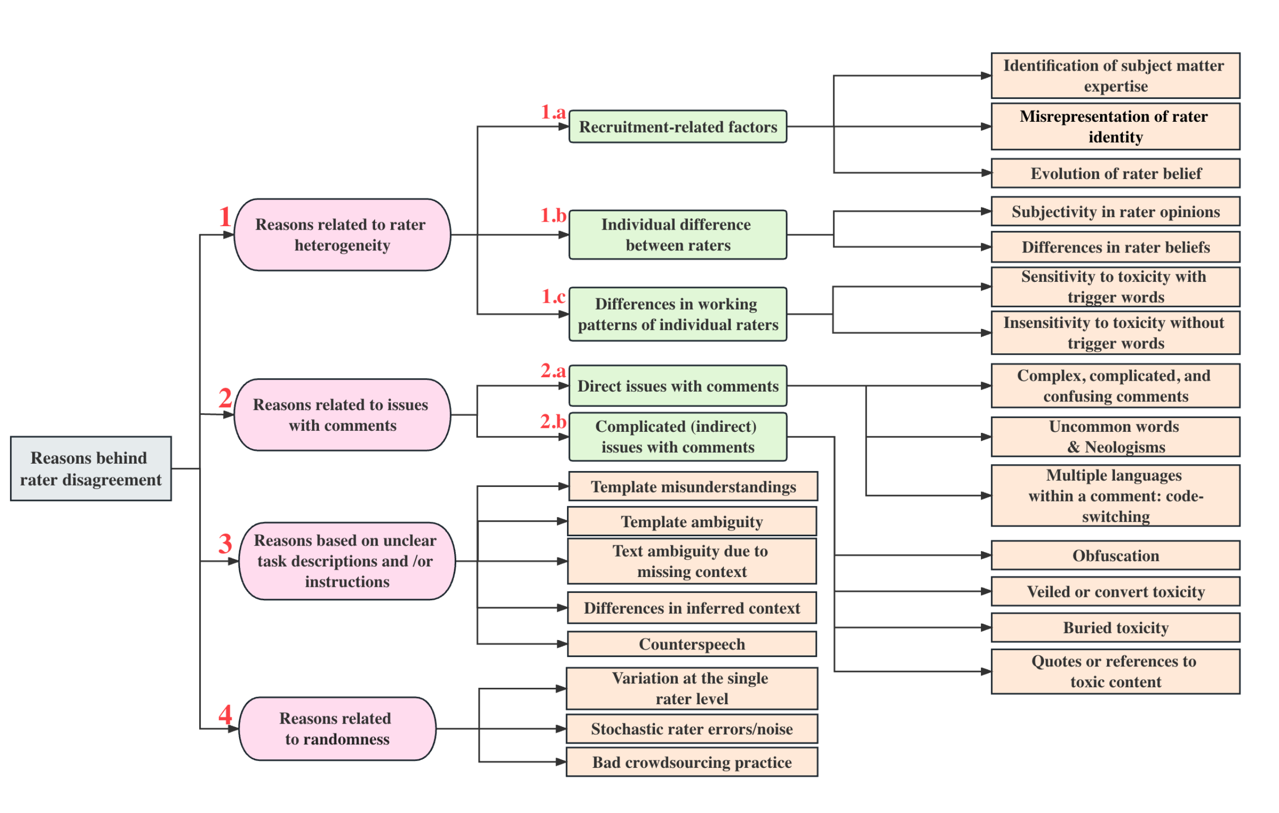
Disagreement deconvolution is built on probabilistic graph modeling:
- Estimate how often an annotator returns non-primary labels, $p_\text{flip}$
- For each sample, compute an adjusted primary-label distribution $p^*$ based on $p_\text{flip}$
- Sample from $p^*$ to construct a new test set.
- Evaluate performance metrics against the new test set.
For $C$-category classification, the sampling procedure of the generative model is defined as follows:
Given the true $p(y\mid x)$ and $p_\text{flip}$, which can be estimated from the data, we update the label distribution of primary labels:
A new test set sampled from $p^*(y \mid x)$ represents the primary labels with individual inconsistency noise removed. This can be used for evaluation as a noise-free test set.
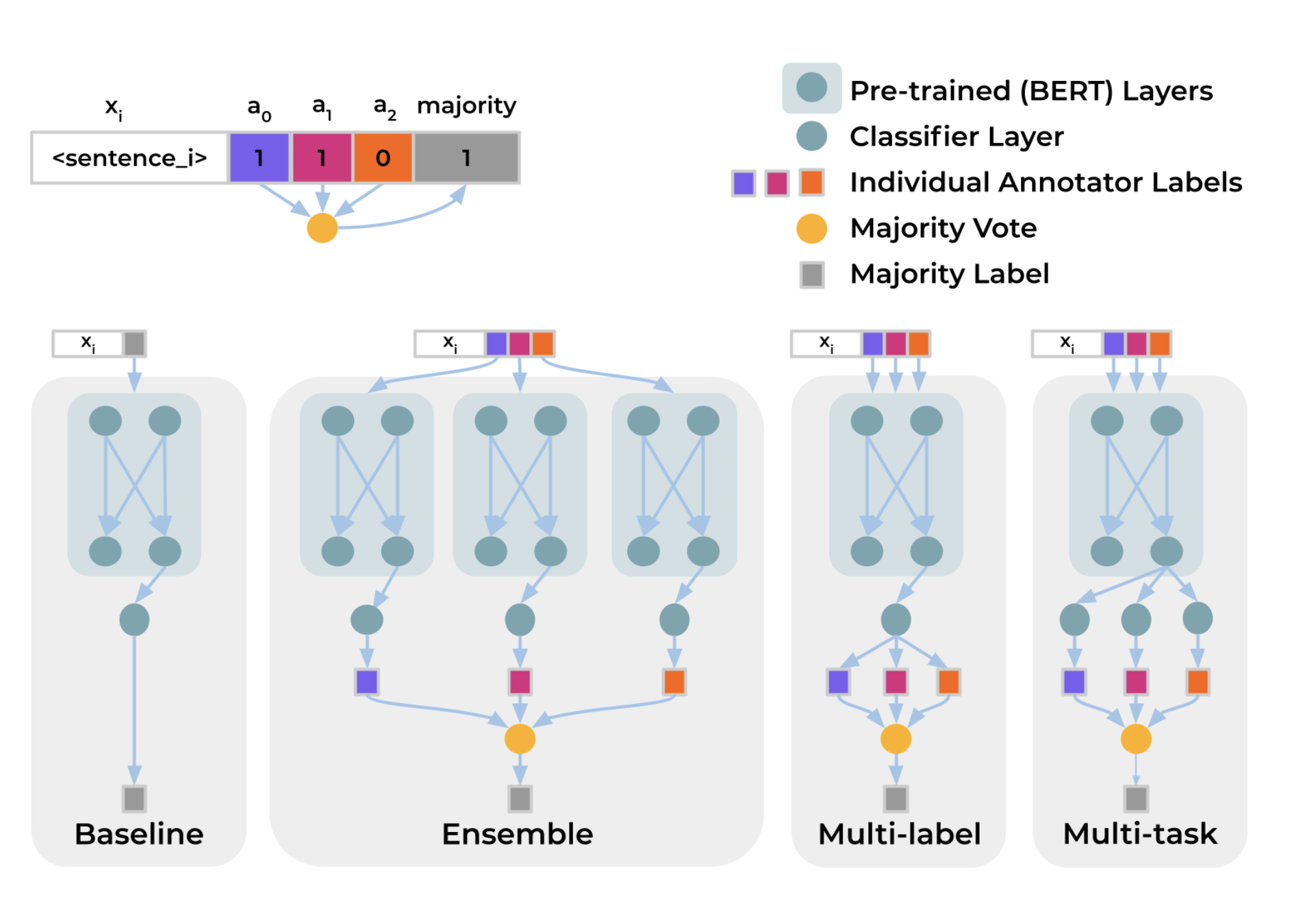
To model systematic disagreement among annotators while learning label predictors, Davani et al. (2021) experimented with a multi-annotator approach in which predicting each annotator’s labels is treated as a separate sub-task. Consider a classification task defined over an annotated dataset $D=(X, A, Y)$, where $X$ is the set of text instances, $A$ is the set of annotators, and $Y$ is the annotation matrix. $y_{ij} \in Y$ denotes a binary label assigned by $a_j \in A$ to sample $x_i \in X$. The majority vote for $x_i$ is denoted by $\bar{y}_{i,}$. The experiment trains a classification head on top of a pre-trained BERT model and compares four setups:
- Baseline: Predict the majority vote $\bar{y}_i$ directly, without using the full annotation matrix $Y$.
- Ensemble: Train one model per annotator to predict $y_{ij}$, then aggregate predictions via majority vote.
- Multi-label: Predict $\vert A \vert$ labels representing all annotators’ labels for each sample $\langle y_{i1}, \dots, y_{i\vert A \vert} \rangle$ using a shared MLP layer, then aggregate outputs.
- Multi-task: Similar to multi-label, but each annotator’s prediction head has a separate MLP layer, allocating additional compute to learn differences among annotators.
Experiments on the GHC (Gab Hate Corpus) dataset showed that the multi-task model achieves the best F1 score. It also naturally provides an uncertainty estimate for predictions that correlates with annotation disagreement.
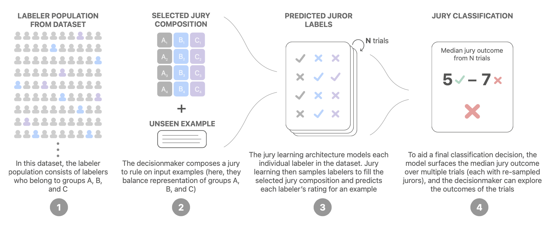
Jury Learning (Gordon et al. 2022) mirrors the jury process by modeling annotators’ labeling behavior conditioned on their characteristics. Starting from a dataset that includes both labels and demographic characteristics for each labeler, a model is trained to predict the labels provided by each individual annotator, where each annotator is treated as a potential juror. At decision time, practitioners can specify the composition of a juror group, which determines a sampling strategy. The final decision is then produced by aggregating labels from jurors across multiple trials.
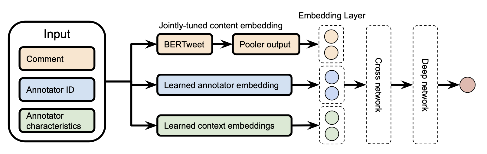
The jury learning model uses a DCN (Deep & Cross network), a model commonly used in recommendation settings, and it is trained jointly to learn a comment embedding, an annotator embedding, and a group embedding (annotator characteristics). Text content is processed by a pre-trained BERT that is also jointly fine-tuned, but for a shorter duration to avoid overfitting.
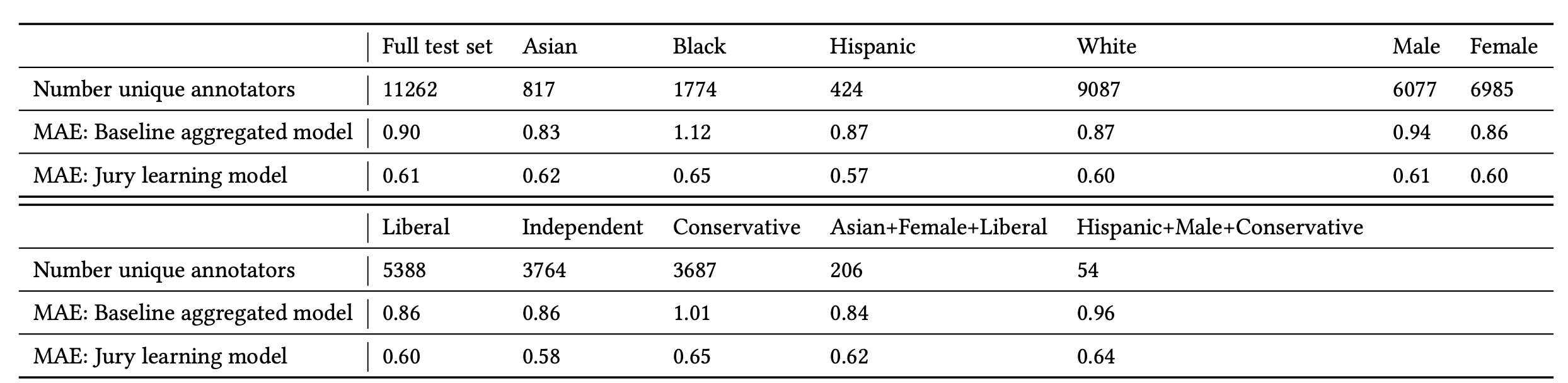
The experiments were conducted on the toxicity diversity dataset, comparing jury learning against a baseline that fine-tunes BERT to predict an individual annotator’s label without metadata. Performance is reported using MAE (mean absolute error). Jury learning consistently outperforms the annotator-agnostic baseline on the full test set and on each group segment.
Data Quality ↔ Model Training
After a dataset is constructed, many methods can identify mislabeled examples by analyzing training dynamics. Note that the focus here is specifically on methods that detect and exclude data points with potentially incorrect labels, not on how to train a model with noisy data.
Influence Functions
Influence functions are a classic tool from robust statistics (Hampel, 1974) for quantifying how individual training points affect a fitted model by describing how model parameters change when a training point is upweighted by an infinitesimal amount. Koh & Liang (2017) introduced this concept for deep neural networks.
Given $n$ training examples, $z_i = (x_i, y_i)$ for $i =1, \dots, n$, model parameters $\theta$ are optimized by minimizing a loss: $\hat{\theta} = \arg\min_{\theta \in \Theta} \frac{1}{n}\sum_{i=1}^n \mathcal{L}(z_i, \theta)$. The parameter change after removing a single training point $z$ is denoted $\hat{\theta}_{-z} - \hat{\theta}$ where $\hat{\theta}_{-z} = \arg\min_{\theta \in \Theta} \frac{1}{n} \sum_{z_i \neq z} \mathcal{L}(z_i, \theta)$. Computing this exactly for every sample is prohibitively expensive. An approximation instead considers the parameter change induced by applying a small upweight $\epsilon$ to $z$. By definition, the influence of upweighting $z$ by $\epsilon$ is:
where $\hat{\theta}_{\epsilon,z} = \arg\min_{\theta \in \Theta} \frac{1}{n}\sum_{i=1}^n \mathcal{L}(z_i, \theta) + \epsilon L(z, \theta)$ and $\mathbf{H}^{-1}_{\hat{\theta}} = \frac{1}{n}\sum_{i=1}^n \nabla^2_\theta \mathcal{L}(z_i, \hat{\theta})$. Removing a data point $x$ is equivalent to upweighting it by $\epsilon = -\frac{1}{n}$, and therefore $\hat{\theta}_{-z} - \hat{\theta} \approx -\frac{1}{n} \mathcal{I}_{\text{up,params}}(z)$.
The influence of upweighting $z$ on the loss at a test point $z_\text{test}$ is derived via the chain rule:
With this closed-form expression, influence functions allow us to estimate the effect of a single data point on model parameters and test loss, approximating leave-one-out retraining without explicitly retraining for each removal. To detect mislabeled data, we can compute $\mathcal{I}_\text{up,loss}(z_i, z_i)$, which approximates the prediction error on $z_i$ if $z_i$ is removed from the training set.
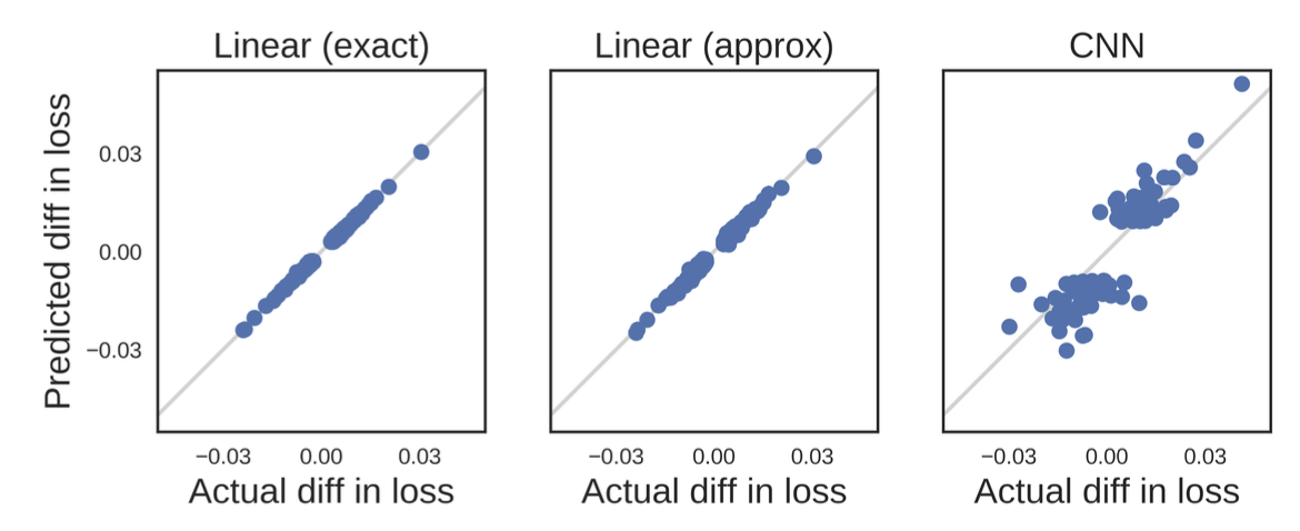
Even with a closed form, influence functions remain difficult to scale because computing the inverse Hessian vector product is challenging. Grosse et al. (2023) experimented with the EK-FAC (Eigenvalue-corrected Kronecker-Factored Approximate Curvature; George et al. 2018) approximation as an alternative.
Prediction Changes during Training
Another family of approaches tracks how model predictions change during training to detect examples that appear difficult for the model to learn. Data Maps (Swayamdipta et al. 2020) track two attributes of training dynamics to analyze dataset quality:
- Confidence: The model’s confidence in the true label, defined as the mean predicted probability of the true label across epochs. They also report a coarse-grained measure, “correctness,” defined as the fraction of epochs in which the model predicts the correct label.
- Variability: The variation in confidence, defined as the standard deviation of the predicted probability of the true label across epochs.
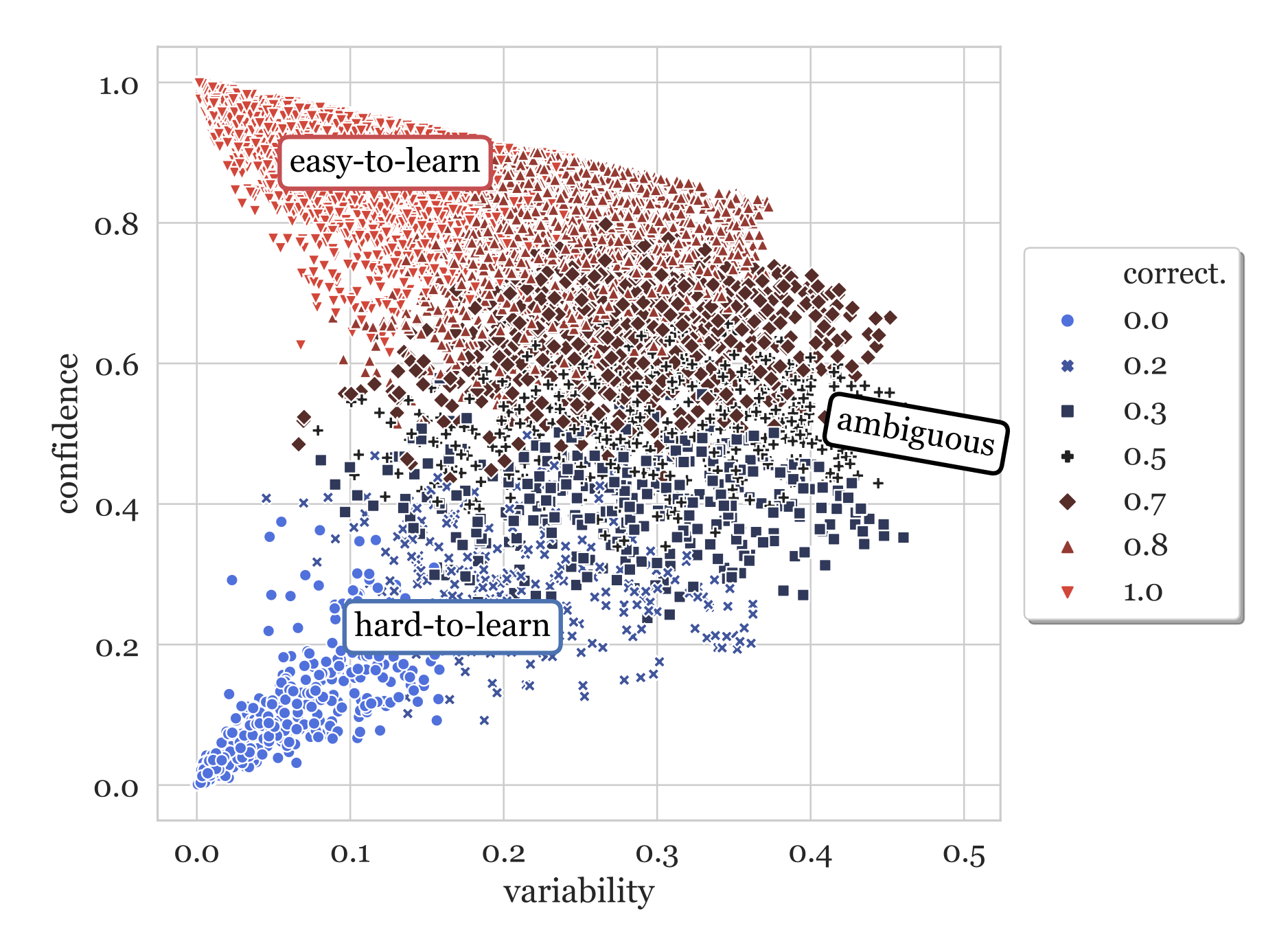
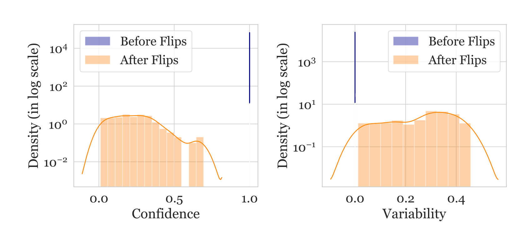
Hard-to-learn examples (low confidence, low variability) are more likely to be mislabeled. In an experiment on the WinoGrande dataset with 1% of labels flipped, retraining caused flipped instances to shift toward lower-confidence and slightly higher-variability regions, suggesting that hard-to-learn areas contain mislabeled examples. Based on this observation, one can train a classifier using equal numbers of flipped-label and clean examples, using only the confidence score (it is unclear why the paper did not use both confidence and variability as features). This simple noise classifier can then be applied to the original dataset to flag potentially mislabeled instances.
It is important not to treat every hard-to-learn example as incorrect. The paper instead hypothesizes that two categories, ambiguous samples (high variability) and hard-to-learn samples (low confidence, low variability), are particularly informative for learning. Experiments show that these samples support out-of-distribution (OOD) generalization and can yield better OOD evaluation performance, even relative to training on the full dataset (100%).
To examine whether neural networks tend to forget information they have already learned, Toneva et al. (2019) propose the following experiment. They monitor the model’s prediction for each example throughout training and count how often each example transitions from correct to incorrect classification, or from incorrect to correct. Based on these transitions, examples can be grouped as follows:
- Forgettable (redundant) samples: the predicted class label changes across training epochs.
- Unforgettable samples: the class label assignment remains consistent across training epochs, meaning the example is never forgotten once it has been learned.
They observe that many training examples are unforgettable and, once learned, are never forgotten. In contrast, examples with noisy labels, or images containing “uncommon” features (making them visually difficult to classify), are among the most frequently forgotten. Their experiments further validate empirically that removing unforgettable examples can be done safely, without degrading model performance.
In their implementation, a forgetting event is counted only when an example appears in the current training batch. In other words, forgetting is computed across repeated presentations of the same example in subsequent mini-batches. The per-example forgetting counts are fairly stable across random seeds, and forgettable examples show a mild tendency to be learned for the first time later in training. Forgetting events are also reported to transfer across the training period and across architectures.
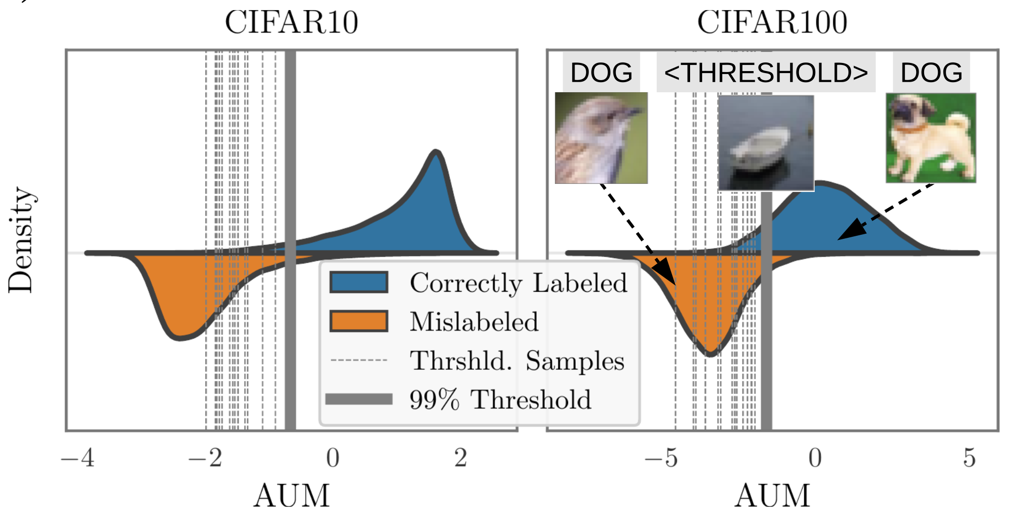
Pleiss, et al. (2020) introduce AUM (Area under the Margin), a method for detecting incorrect labels under the following assumption. For example, if an image of a BIRD is mistakenly labeled as DOG, gradient updates driven by other BIRD images will encourage the model to generalize in a way consistent with the BIRD class, while the (incorrect) DOG label supplies a supervised signal pushing the update in the opposite direction. As a result, gradient updates reflect a tension between generalization and (wrong) prediction signals.
Given a classification dataset $(\mathbf{x}, y) \in \mathcal{D}_\text{train}$, let $z^{(t)}_i(\mathbf{x}) \in \mathbb{R}$ be the logit corresponding to class $i$ at epoch $t$. The margin at epoch $t$ is defined as the difference between the assigned logit and the next-largest logit:
A negative margin indicates an incorrect prediction, whereas a large positive margin indicates high confidence in a correct prediction. The central hypothesis is that mislabeled examples tend to exhibit smaller margins than correctly labeled ones, due to the SGD-driven generalization pressure coming from other samples.
To choose a threshold, they add synthetic examples, referred to as “threshold samples,” and use them to set the cutoff:
- Create a subset of threshold samples $\mathcal{D}_\text{thr}$. If there are $N$ training samples for $C$ classes, randomly sample $N/(C+1)$ samples and change all of their labels to a new, fake class $C+1$.
- Merge the threshold samples into the original dataset: $\mathcal{D}’ = { (\mathbf{x}, C+1): \mathbf{x} \in \mathcal{D}_\text{thr}} \cup (\mathcal{D} \setminus\mathcal{D}_\text{thr})$;
- Train the model on $\mathcal{D}’$ and compute the AUM for all data;
- Compute the threshold $\alpha$ as the 99th percentile of the AUM values among threshold samples;
- Detect mislabeled data using $\alpha$ a threshold: ${(\mathbf{x}, y) \in \mathcal{D} \setminus \mathcal{D}_\text{thr}: \text{AUM}_{\mathbf{x}, y} \leq \alpha}$
Noisy Cross-Validation
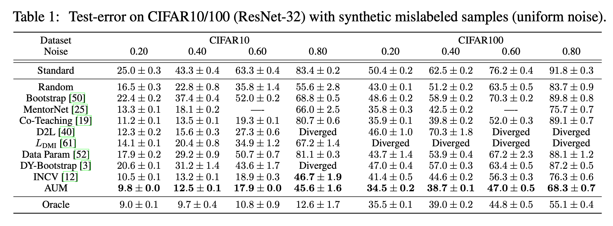
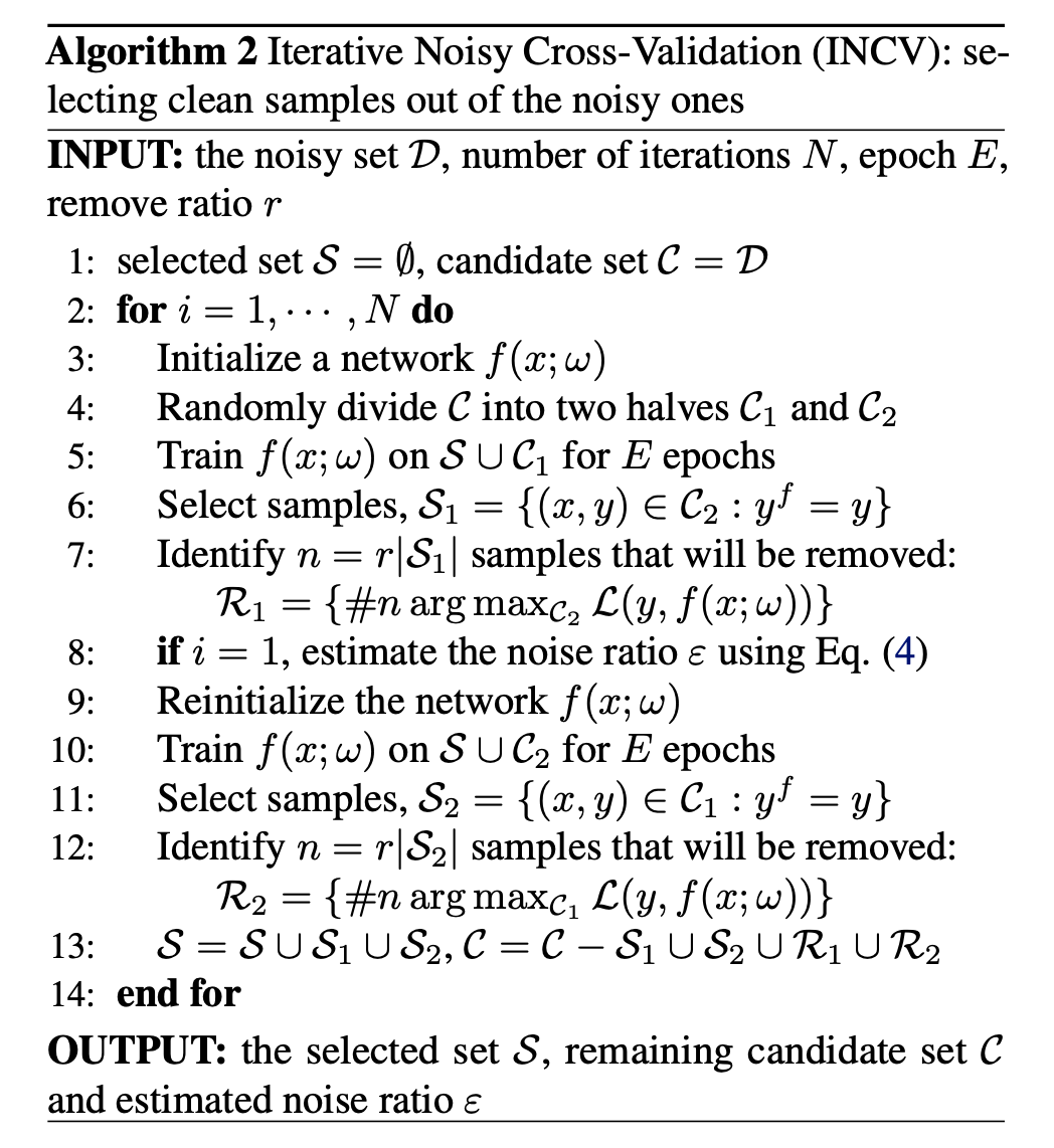
NCV (Noisy Cross-Validation) (Chen et al. 2019) randomly splits the dataset into two halves, then marks an example as “clean” if its label matches the label predicted by a model trained only on the other half. These clean examples are treated as more reliable. INCV (Iterative Noisy Cross-Validation) applies NCV iteratively, progressively adding more clean examples into the trusted candidate set $\mathcal{C}$ while removing additional noisy examples.
Citation
Cited as:
Weng, Lilian. (Feb 2024). “Thinking about High-Quality Human Data”. Lil’Log. https://lilianweng.github.io/posts/2024-02-05-human-data-quality/.
Or
@article{weng2024humandata,
  title   = "Thinking about High-Quality Human Data",
  author  = "Weng, Lilian",
  journal = "lilianweng.github.io",
  year    = "2024",
  month   = "Feb",
  url     = "https://lilianweng.github.io/posts/2024-02-05-human-data-quality/"
}
References
[1] Francis Galton “Vox populi” Nature 75, 450-451 (1907).
[2] Sambasivan et al. “Everyone wants to do the model work, not the data work”: Data Cascades in High-Stakes AI" CHI 2021
[3] Chris Callison-Burch. “Fast, Cheap, and Creative: Evaluating Translation Quality Using Amazon’s Mechanical Turk” EMNLP 2009
[4] Rottger et al. “Two Contrasting Data Annotation Paradigms for Subjective NLP Tasks” NAACL 2022.
[5] Aroyo & Welty “Truth Is a Lie: Crowd Truth and the Seven Myths of Human Annotation” AI Magazine 36.1: 15-24 (2015).
[6] Hovy et al. “Learning Whom to Trust with MACE” NAACL-HLT 2013.
[7] Wang et al. “All that Agrees Is Not Gold: Evaluating Ground Truth Labels and Dialogue Content for Safety” 2023.
[8] Zhang et al. “A Taxonomy of Rater Disagreements: Surveying Challenges & Opportunities from the Perspective of Annotating Online Toxicity” arXiv preprint arXiv:2311.04345 (2023).
[9] Davani et al. “Dealing with disagreements: Looking beyond the majority vote in subjective annotations” ACL 2022.
[10] Gordon et al. “Jury Learning: Integrating Dissenting Voices into Machine Learning Models” CHI 2022.
[11] Gordon et al. “The Disagreement Deconvolution: Bringing Machine Learning Performance Metrics In Line With Reality” CHI 2021
[12] Daniel et al. 2018 “Quality Control in Crowdsourcing: A Survey of Quality Attributes, Assessment Techniques, and Assurance Actions” ACM Computing Surveys (CSUR), 51(1), 1-40 (2018).
[13] Koh & Liang. “Understanding Black-box Predictions via Influence Functions” ICML 2017.
[14] Grosse et al. “Studying Large Language Model Generalization with Influence Functions” arXiv preprint arXiv:2308.03296 (2023).
[15] Swayamdipta et al. “Dataset Cartography: Mapping and Diagnosing Datasets with Training Dynamics” EMNLP 2020.
[16] Toneva, et al. “An Empirical Study of Example Forgetting during Deep Neural Network Learning” ICLR 2019.
[17] Pleiss, et al. “Identifying Mislabeled Data using the Area Under the Margin Ranking” NeuriPS 2020.
[18] Chen et al. “Understanding and utilizing deep neural networks trained with noisy labels” ICML 2019.