Object Detection for Dummies Part 1: Gradient Vectors, HOG, and SS
I have never worked in computer vision, and I do not understand how the “magic” works when an autonomous car is configured to distinguish a stop sign from a pedestrian wearing a red hat. To motivate myself to study the mathematics behind object recognition and detection algorithms, I am writing a series of posts on this topic, “Object Detection for Dummies.” This first post begins with very basic concepts in image processing and introduces several methods for image segmentation. It does not cover deep neural networks. Deep learning models for object detection and recognition will be discussed in Part 2 and Part 3.
· 15 min read · Curated and presented by Arthur Sedek
I have never worked in computer vision, and I previously had little intuition for how an autonomous car can reliably distinguish a stop sign from a pedestrian wearing a red hat. To motivate myself to learn the mathematics behind object recognition and detection, I am writing a set of posts under the title “Object Detection for Dummies.” This first post begins with very basic image processing ideas and a few image segmentation methods. It does not cover deep neural networks yet. Deep learning models for object detection and recognition are discussed in Part 2 and Part 3.
Disclaimer: When I started, I used “object recognition” and “object detection” interchangeably. I do not think they are identical: object recognition is primarily about determining whether an object exists in an image, while object detection also requires identifying where the object is. That said, the two topics are tightly connected, and many object recognition algorithms provide the groundwork for detection.
Links to all posts in the series: [Part 1] [Part 2] [Part 3] [Part 4].
Image Gradient Vector
Before going further, it is important to distinguish the following terms. They are closely related and often conflated, but they are not exactly the same.
| Derivative | Directional Derivative | Gradient | |
|---|---|---|---|
| Value type | Scalar | Scalar | Vector |
| Definition | The rate of change of a function $f(x,y,z,…)$ at a point $(x_0,y_0,z_0,…)$, which is the slope of the tangent line at the point. | The instantaneous rate of change of $f(x,y,z, …)$ in the direction of an unit vector $\vec{u}$. | It points in the direction of the greatest rate of increase of the function, containing all the partial derivative information of a multivariable function. |
In image processing, we often want to determine the direction in which colors change from one extreme to another (for example, from black to white in a grayscale image). To do that, we measure the “gradient” of pixel intensities. Because images consist of discrete pixels and each pixel is an indivisible unit, the image gradient is also discrete.
The image gradient vector is defined per pixel and captures intensity changes along both the x-axis and the y-axis. This definition mirrors the gradient of a continuous multivariable function, which is a vector composed of the partial derivatives with respect to each variable. Let f(x, y) denote the pixel intensity at location (x, y). The gradient vector at pixel (x, y) is defined as:
The $\frac{\partial f}{\partial x}$ term is the partial derivative in the x direction. It is computed as the intensity difference between the adjacent pixels to the left and right of the target pixel, f(x+1, y) - f(x-1, y). Likewise, the $\frac{\partial f}{\partial y}$ term is the partial derivative in the y direction, computed as f(x, y+1) - f(x, y-1), which is the intensity difference between the pixels immediately above and below the target.
Two key attributes are commonly derived from an image gradient:
- Magnitude: the L2 norm of the vector, $g = \sqrt{ g_x^2 + g_y^2 }$.
- Direction: the arctangent of the ratio between the two directional partial derivatives, $\theta = \arctan{(g_y / g_x)}$.
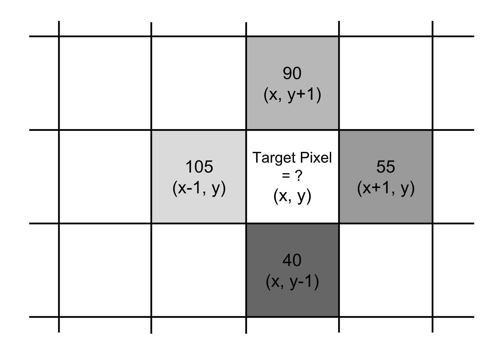
The gradient vector in the example is:
Therefore:
- the magnitude is $\sqrt{50^2 + (-50)^2} = 70.7107$, and
- the direction is $\arctan{(-50/50)} = -45^{\circ}$.
Computing gradients by iterating over every pixel is inefficient. In practice, the same computation is expressed as applying a convolution operator to the full image matrix, denoted as $\mathbf{A}$, using specially designed convolution kernels.
Consider the x direction in the example in Fig 1. Using the kernel $[-1,0,1]$ sliding across the x-axis (where $\ast$ denotes the convolution operator):
Similarly, for the y direction, we use the kernel $[+1, 0, -1]^\top$:
Try this in python:
import numpy as np
import scipy.signal as sig
data = np.array([[0, 105, 0], [40, 255, 90], [0, 55, 0]])
G_x = sig.convolve2d(data, np.array([[-1, 0, 1]]), mode='valid')
G_y = sig.convolve2d(data, np.array([[-1], [0], [1]]), mode='valid')
These two functions return array([[0], [-50], [0]]) and array([[0, 50, 0]]), respectively. (Note that in the numpy array representation, 40 appears before 90, so -1 is listed before 1 in the kernel accordingly.)
Common Image Processing Kernels
Prewitt operator: Instead of using only the four directly adjacent neighbors, the Prewitt operator incorporates all eight surrounding pixels to produce smoother results.
Sobel operator: To place more emphasis on directly adjacent pixels, those neighbors are assigned higher weights.
Kernels can be designed for different objectives, including edge detection, blurring, sharpening, and many others. See this wiki page for additional examples and references.
Example: Manu in 2004
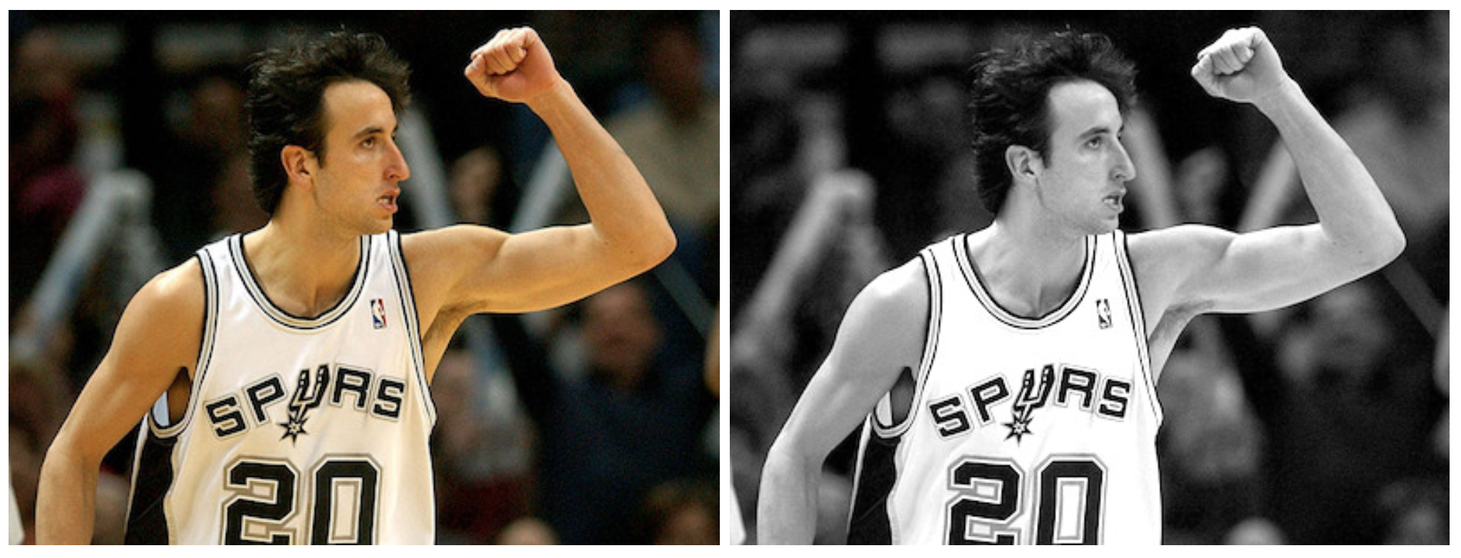
Let’s run a simple experiment on a photo of Manu Ginobili in 2004 [[Download Image]({{ ‘/assets/data/manu-2004.jpg’ | relative_url }}){:target="_blank"}], back when he still had a lot of hair. For simplicity, we first convert the photo to grayscale. For a color image, we would apply the same process independently to each color channel.
import numpy as np
import scipy
import scipy.signal as sig
# With mode="L", we force the image to be parsed in the grayscale, so it is
# actually unnecessary to convert the photo color beforehand.
img = scipy.misc.imread("manu-2004.jpg", mode="L")

# Define the Sobel operator kernels.
kernel_x = np.array([[-1, 0, 1],[-2, 0, 2],[-1, 0, 1]])
kernel_y = np.array([[1, 2, 1], [0, 0, 0], [-1, -2, -1]])

G_x = sig.convolve2d(img, kernel_x, mode='same')
G_y = sig.convolve2d(img, kernel_y, mode='same')

# Plot them!
fig = plt.figure()
ax1 = fig.add_subplot(121)
ax2 = fig.add_subplot(122)

# Actually plt.imshow() can handle the value scale well even if I don't do
# the transformation (G_x + 255) / 2.
ax1.imshow((G_x + 255) / 2, cmap='gray'); ax1.set_xlabel("Gx")
ax2.imshow((G_y + 255) / 2, cmap='gray'); ax2.set_xlabel("Gy")
plt.show()
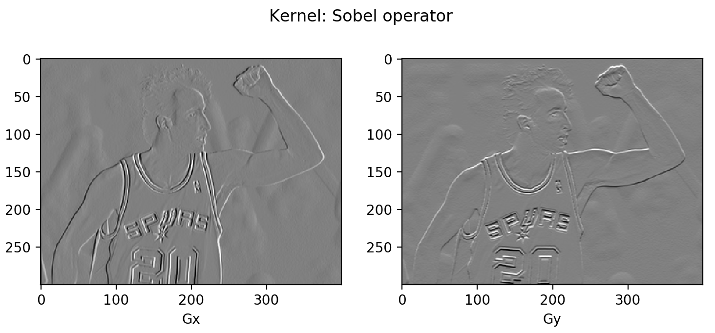
You may notice that much of the output appears gray. This happens because the difference between two pixels falls within [-255, 255], and for display we must map values back into [0, 255]. A simple linear transformation, ($\mathbf{G}$ + 255)/2, maps zeros (that is, regions with constant intensity and therefore no gradient change) to 125, which is displayed as gray.
Histogram of Oriented Gradients (HOG)
The Histogram of Oriented Gradients (HOG) is an efficient feature extraction approach that summarizes pixel-level information for use in an object recognition classifier. With image gradient vectors in hand, the mechanics of HOG are straightforward. Let’s walk through the process.
How HOG works
-
Preprocess the image, including resizing and color normalization.
-
Compute the gradient vector at every pixel, along with its magnitude and direction.
-
Partition the image into 8x8 pixel cells. Within each cell, the magnitude values for these 64 pixels are binned and accumulated into 9 buckets based on unsigned direction (no sign, so 0-180 degrees rather than 0-360 degrees; this is a practical choice supported by empirical experiments).
For improved robustness, if a pixel’s gradient direction lies between two buckets, its magnitude is not assigned entirely to the nearest bucket. Instead, it is split proportionally across the two neighboring buckets. For example, if a pixel’s gradient magnitude is 8 and its direction is 15 degrees, then it falls between the 0-degree and 20-degree buckets. We would assign 2 to the 0-degree bucket and 6 to the 20-degree bucket.
This configuration makes the histogram more stable under small image distortions.
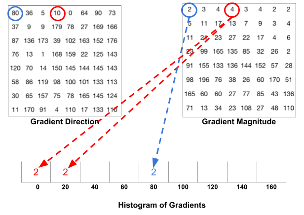
- Next, slide a 2x2-cell block (that is, 16x16 pixels) across the image. For each block, concatenate the four cell histograms into a 36-dimensional vector, then normalize it to have unit weight. The final HOG feature vector is formed by concatenating all block vectors. This feature representation can then be used as input to a classifier such as an SVM for object recognition tasks.
Example: Manu in 2004
Let’s reuse the same image from the previous section. Recall that we already computed $\mathbf{G}_x$ and $\mathbf{G}_y$ for the entire image.
N_BUCKETS = 9
CELL_SIZE = 8  # Each cell is 8x8 pixels
BLOCK_SIZE = 2  # Each block is 2x2 cells

def assign_bucket_vals(m, d, bucket_vals):
    left_bin = int(d / 20.)
    # Handle the case when the direction is between [160, 180)
    right_bin = (int(d / 20.) + 1) % N_BUCKETS
    assert 0 <= left_bin < right_bin < N_BUCKETS

    left_val= m * (right_bin * 20 - d) / 20
    right_val = m * (d - left_bin * 20) / 20
    bucket_vals[left_bin] += left_val
    bucket_vals[right_bin] += right_val

def get_magnitude_hist_cell(loc_x, loc_y):
    # (loc_x, loc_y) defines the top left corner of the target cell.
    cell_x = G_x[loc_x:loc_x + CELL_SIZE, loc_y:loc_y + CELL_SIZE]
    cell_y = G_y[loc_x:loc_x + CELL_SIZE, loc_y:loc_y + CELL_SIZE]
    magnitudes = np.sqrt(cell_x * cell_x + cell_y * cell_y)
    directions = np.abs(np.arctan(cell_y / cell_x) * 180 / np.pi)

    buckets = np.linspace(0, 180, N_BUCKETS + 1)
    bucket_vals = np.zeros(N_BUCKETS)
    map(
        lambda (m, d): assign_bucket_vals(m, d, bucket_vals),
        zip(magnitudes.flatten(), directions.flatten())
    )
    return bucket_vals

def get_magnitude_hist_block(loc_x, loc_y):
    # (loc_x, loc_y) defines the top left corner of the target block.
    return reduce(
        lambda arr1, arr2: np.concatenate((arr1, arr2)),
        [get_magnitude_hist_cell(x, y) for x, y in zip(
            [loc_x, loc_x + CELL_SIZE, loc_x, loc_x + CELL_SIZE],
            [loc_y, loc_y, loc_y + CELL_SIZE, loc_y + CELL_SIZE],
        )]
    )
The following code simply invokes the functions to build a histogram and plot it.
# Random location [200, 200] as an example.
loc_x = loc_y = 200

ydata = get_magnitude_hist_block(loc_x, loc_y)
ydata = ydata / np.linalg.norm(ydata)

xdata = range(len(ydata))
bucket_names = np.tile(np.arange(N_BUCKETS), BLOCK_SIZE * BLOCK_SIZE)

assert len(ydata) == N_BUCKETS * (BLOCK_SIZE * BLOCK_SIZE)
assert len(bucket_names) == len(ydata)

plt.figure(figsize=(10, 3))
plt.bar(xdata, ydata, align='center', alpha=0.8, width=0.9)
plt.xticks(xdata, bucket_names * 20, rotation=90)
plt.xlabel('Direction buckets')
plt.ylabel('Magnitude')
plt.grid(ls='--', color='k', alpha=0.1)
plt.title("HOG of block at [%d, %d]" % (loc_x, loc_y))
plt.tight_layout()
In the code above, I use the block whose top-left corner is at [200, 200] as an example. The figure below shows the final normalized histogram for that block. You can modify the code to change the block location, for example, by using a sliding window to enumerate blocks.
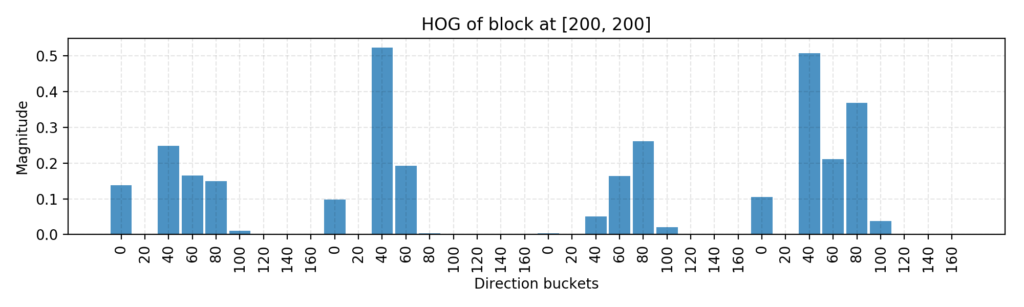
This code is primarily intended to illustrate the computation workflow. In practice, many off-the-shelf libraries already provide HOG implementations, including OpenCV, SimpleCV, and scikit-image.
Image Segmentation (Felzenszwalb’s Algorithm)
When an image contains multiple objects (as is the case for almost all real-world photos), it is often useful to identify regions that may contain the target object. Doing so allows classification to be performed more efficiently.
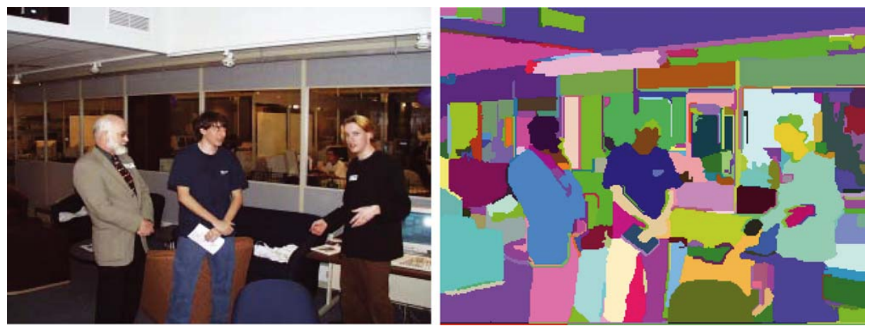
Felzenszwalb and Huttenlocher (2004) proposed a graph-based method to segment an image into similar regions. This method is also used to initialize Selective Search (a widely used region proposal algorithm) that we will discuss later.
Assume we represent an input image as an undirected graph $G=(V, E)$. Each vertex $v_i \in V$ corresponds to a pixel. An edge $e = (v_i, v_j) \in E$ connects two vertices $v_i$ and $v_j$, and its weight $w(v_i, v_j)$ quantifies the dissimilarity between $v_i$ and $v_j$. Dissimilarity can be defined over dimensions such as color, location, intensity, and so on. Larger weights indicate less similar pixels. A segmentation solution $S$ is a partition of $V$ into multiple connected components, $\{C\}$. Intuitively, similar pixels should fall into the same component, while dissimilar pixels should be assigned to different components.
Graph Construction
Two common strategies can be used to construct a graph from an image.
- Grid Graph: Each pixel is connected only to its surrounding neighbours (8 adjacent cells in total). The edge weight is the absolute difference between the pixels’ intensity values.
- Nearest Neighbor Graph: Each pixel is treated as a point in feature space (x, y, r, g, b), where (x, y) denotes pixel location and (r, g, b) denotes RGB color values. The edge weight is the Euclidean distance between the feature vectors of two pixels.
Key Concepts
Before stating the criteria for a good graph partition (that is, an image segmentation), we first introduce a few key concepts:
- Internal difference: $Int(C) = \max_{e\in MST(C, E)} w(e)$, where $MST$ is the minimum spanning tree of the components. A component $C$ remains connected even after removing all edges with weights < $Int(C)$.
- Difference between two components: $Dif(C_1, C_2) = \min_{v_i \in C_1, v_j \in C_2, (v_i, v_j) \in E} w(v_i, v_j)$. $Dif(C_1, C_2) = \infty$ if there is no edge in-between.
- Minimum internal difference: $MInt(C_1, C_2) = min(Int(C_1) + \tau(C_1), Int(C_2) + \tau(C_2))$, where $\tau(C) = k / \vert C \vert$ ensures a meaningful threshold for inter-component differences. With a larger $k$, the algorithm is more likely to produce larger components.
Segmentation quality is evaluated using a pairwise region comparison predicate defined for two regions $C_1$ and $C_2$:
Only when this predicate evaluates to True do we treat the two regions as independent components. Otherwise, the segmentation is considered overly fine, and the regions likely should be merged.
How Image Segmentation Works
The algorithm proceeds bottom-up. Given $G=(V, E)$ and $|V|=n, |E|=m$:
- Sort all edges by weight in ascending order, denoted as $e_1, e_2, \dots, e_m$.
- Initialize by placing each pixel in its own component, yielding $n$ components.
- Repeat for $k=1, \dots, m$:
- Let the segmentation state at step $k$ be $S^k$.
- Select the k-th edge in the sorted list, $e_k = (v_i, v_j)$.
- If $v_i$ and $v_j$ are already in the same component, take no action, and therefore $S^k = S^{k-1}$.
- If $v_i$ and $v_j$ lie in two different components $C_i^{k-1}$ and $C_j^{k-1}$ in segmentation $S^{k-1}$, merge them into a single component if $w(v_i, v_j) \leq MInt(C_i^{k-1}, C_j^{k-1})$; otherwise, do nothing.
If you would like to see the proof of the segmentation properties and the argument for why a valid segmentation always exists, please consult the paper.
Example: Manu in 2013
In this example, I use a photo of Manu Ginobili in 2013 [[Image]({{ ‘/assets/data/manu-2013.jpg’ | relative_url }})], at a time when his bald spot had become quite prominent. For simplicity, we again use the grayscale version of the image.
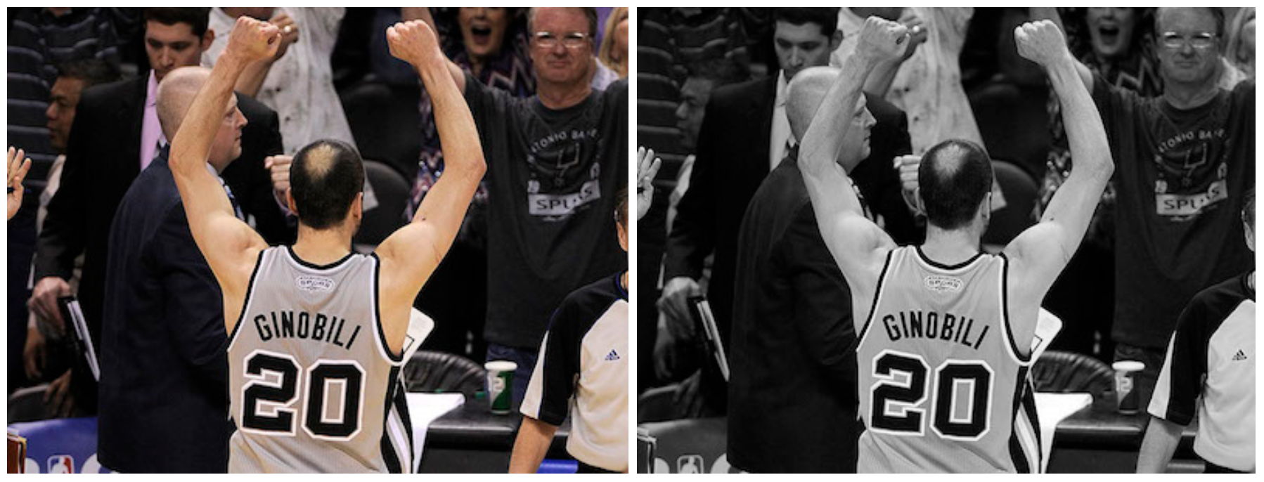
Instead of implementing the algorithm from scratch, we apply skimage.segmentation.felzenszwalb to this image.
import skimage.segmentation
from matplotlib import pyplot as plt

img2 = scipy.misc.imread("manu-2013.jpg", mode="L")
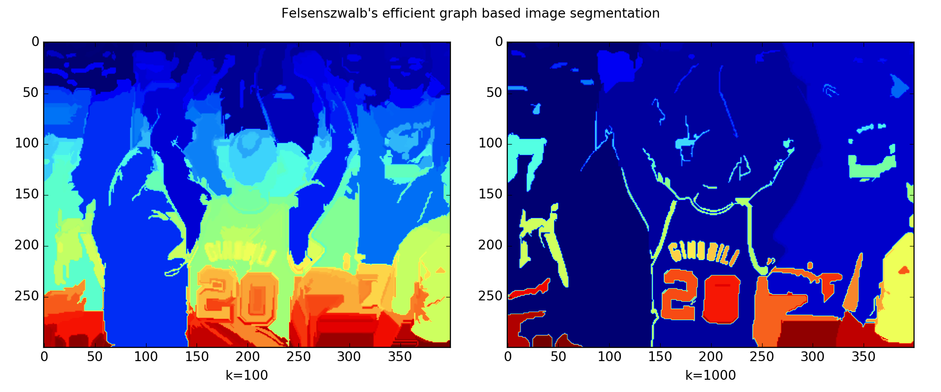
segment_mask1 = skimage.segmentation.felzenszwalb(img2, scale=100)
segment_mask2 = skimage.segmentation.felzenszwalb(img2, scale=1000)

fig = plt.figure(figsize=(12, 5))
ax1 = fig.add_subplot(121)
ax2 = fig.add_subplot(122)
ax1.imshow(segment_mask1); ax1.set_xlabel("k=100")
ax2.imshow(segment_mask2); ax2.set_xlabel("k=1000")
fig.suptitle("Felsenszwalb's efficient graph based image segmentation")
plt.tight_layout()
plt.show()
The code runs two configurations of Felzenszwalb’s algorithm. The left result, k=100, produces a finer-grained segmentation with smaller regions, in which Manu’s bald spot is separated out. The right result, k=1000, produces a coarser segmentation with regions that tend to be larger.
Selective Search
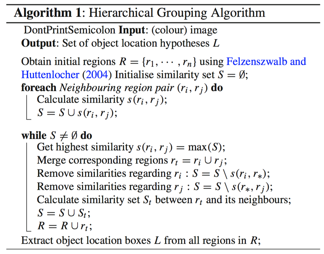
Selective Search is a widely used algorithm for generating region proposals that may contain objects. It builds on the output of image segmentation and performs bottom-up hierarchical grouping using region-based characteristics (NOTE: not merely attributes of individual pixels).
How Selective Search Works
- Initialization: apply Felzenszwalb and Huttenlocher’s graph-based image segmentation algorithm to produce the initial set of regions.
- Iteratively group regions using a greedy procedure:
- Compute similarities between all neighbouring regions.
- Merge the two most similar regions, then recompute similarities between the merged region and its neighbours.
- Repeat the grouping step (Step 2) until the entire image is represented as a single region.
Configuration Variations
Given two regions $(r_i, r_j)$, Selective Search proposes four complementary similarity measures:
- Color similarity
- Texture: Use an algorithm that performs well for material recognition, such as SIFT.
- Size: Encourage small regions to merge early.
- Shape: Ideally, one region can fill the gap of the other.
By (i) tuning the threshold $k$ in Felzenszwalb and Huttenlocher’s algorithm, (ii) changing the color space, and (iii) selecting different combinations of similarity metrics, we can generate a diverse set of Selective Search strategies. The configuration that yields the highest-quality region proposals uses (i) a mixture of different initial segmentation proposals, (ii) a blend of multiple color spaces, and (iii) a combination of all similarity measures. As expected, this requires balancing quality (model complexity) against speed.
Cited as:
@article{weng2017detection1,
  title   = "Object Detection for Dummies Part 1: Gradient Vector, HOG, and SS",
  author  = "Weng, Lilian",
  journal = "lilianweng.github.io",
  year    = "2017",
  url     = "https://lilianweng.github.io/posts/2017-10-29-object-recognition-part-1/"
}
References
[1] Dalal, Navneet, and Bill Triggs. “Histograms of oriented gradients for human detection.” Computer Vision and Pattern Recognition (CVPR), 2005.
[2] Pedro F. Felzenszwalb, and Daniel P. Huttenlocher. “Efficient graph-based image segmentation.” Intl. journal of computer vision 59.2 (2004): 167-181.
[3] Histogram of Oriented Gradients by Satya Mallick