Object Detection for Dummies Part 3: R-CNN Family
[Updated on 2018-12-20: Removed YOLO from this article. Part 4 will cover multiple fast object detection algorithms, including YOLO.] [Updated on 2018-12-27: Added sections on bbox regression and R-CNN tricks.] In the “Object Detection for Dummies” series, Part 1 covered foundational image-processing concepts, including gradient vectors and HOG. Part 2 then reviewed classic convolutional neural network architecture designs for classification, along with early object-recognition models such as Overfeat and DPM. In this third installment, we will examine a set of models in the R-CNN (“Region-based CNN”) family.
· 13 min read · Curated and presented by Arthur Sedek
[Updated on 2018-12-20: Remove YOLO here. Part 4 will cover multiple fast object detection algorithms, including YOLO.]
[Updated on 2018-12-27: Add bbox regression and tricks sections for R-CNN.]
In the “Object Detection for Dummies” series, we began in Part 1 with foundational image processing concepts such as gradient vectors and HOG. Next, in Part 2, we discussed classic convolutional neural network architectures for classification and introduced early object recognition models, including Overfeat and DPM. In this third post, we review a set of models in the R-CNN (“Region-based CNN”) family.
Links to all the posts in the series: [Part 1] [Part 2] [Part 3] [Part 4].
Here is a list of papers covered in this post ;)
| Model | Goal | Resources |
|---|---|---|
| R-CNN | Object recognition | [paper][code] |
| Fast R-CNN | Object recognition | [paper][code] |
| Faster R-CNN | Object recognition | [paper][code] |
| Mask R-CNN | Image segmentation | [paper][code] |
R-CNN
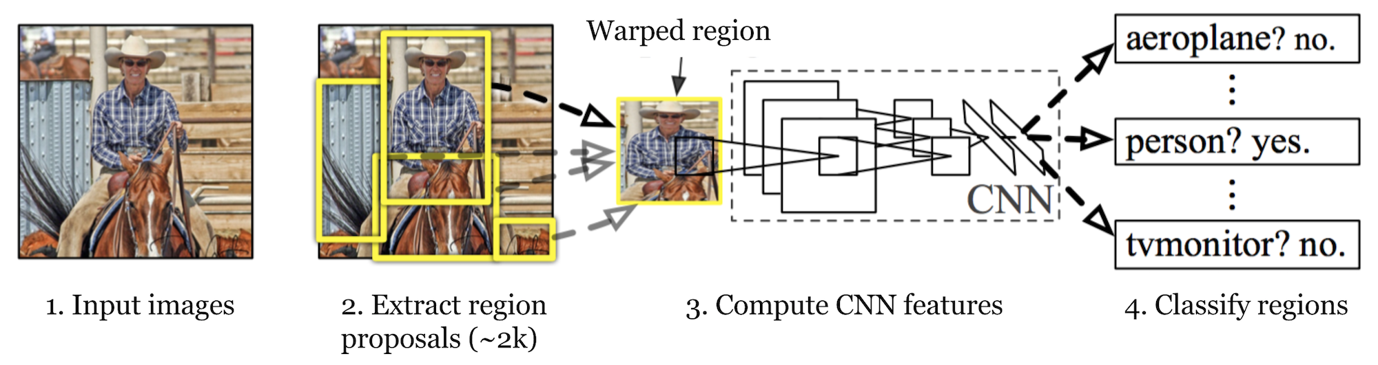
R-CNN (Girshick et al., 2014), short for “Region-based Convolutional Neural Networks,” is built around a two-stage approach. First, it uses selective search to generate a manageable set of object region candidates in the form of bounding boxes (regions of interest, or “RoIs”). Second, it extracts CNN features from each candidate region independently and uses those features for classification.
Model Workflow
At a high level, R-CNN operates as follows:
- Pre-train a CNN on an image classification task, for example, VGG or ResNet trained on the ImageNet dataset. This classification task contains N classes.
NOTE: You can find a pre-trained AlexNet in Caffe Model Zoo. I don’t think you can find it in Tensorflow, but Tensorflow-slim model library provides pre-trained ResNet, VGG, and others.
- Use selective search to propose category-independent regions of interest (approximately 2k candidates per image). These regions vary in size and may contain target objects.
- Warp each region candidate to a fixed size so it can be processed by the CNN.
- Fine-tune the CNN on the warped proposal regions for K + 1 classes. The additional class represents the background (no object of interest). During fine-tuning, use a much smaller learning rate, and oversample positive cases in the mini-batch because most proposed regions are background.
- For each image region, run a forward pass through the CNN to produce a feature vector. Train a binary SVM per class to consume these features.
Positive samples are proposed regions whose IoU (intersection over union) overlap is >= 0.3, and negative samples are all other irrelevant regions. - To reduce localization error, train a regression model that uses CNN features to predict bounding box correction offsets, tightening the predicted detection window.
Bounding Box Regression
Given a predicted bounding box coordinate $\mathbf{p} = (p_x, p_y, p_w, p_h)$ (center coordinate, width, height) and its corresponding ground truth box coordinates $\mathbf{g} = (g_x, g_y, g_w, g_h)$ , the regressor is set up to learn a scale-invariant transformation between the two centers and a log-scale transformation between widths and heights. All transformation functions take $\mathbf{p}$ as input.
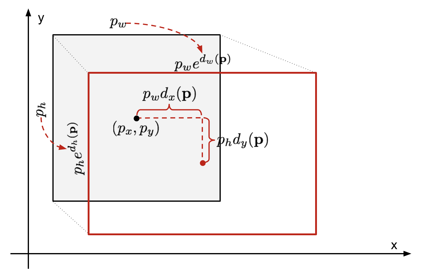
A clear advantage of this parameterization is that the bounding box correction functions, $d_i(\mathbf{p})$ where $i \in \{ x, y, w, h \}$, can take any value in [-∞, +∞]. The learning targets are:
This can be addressed with a standard regression model by minimizing the SSE loss with regularization:
The regularization term is essential, and the RCNN paper selects the best λ via cross validation. Also note that not every predicted bounding box corresponds to a ground truth box. For instance, when there is no overlap, applying bbox regression is not meaningful. Therefore, training the bbox regression model keeps only predicted boxes that have a nearby ground truth box with at least 0.6 IoU.
Common Tricks
Several techniques are commonly used in RCNN and other detection models.
Non-Maximum Suppression
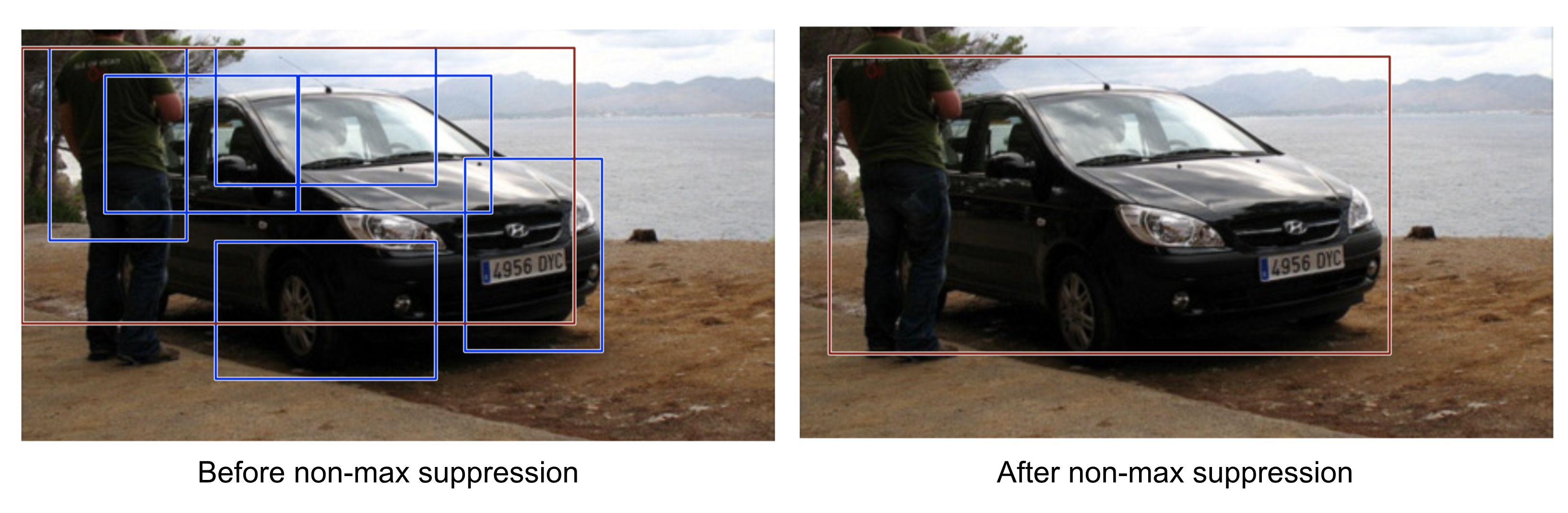
In practice, the model may produce multiple bounding boxes for the same object. Non-maximum suppression helps prevent repeated detections of the same instance. After obtaining a set of matched bounding boxes for a given object category: Sort all the bounding boxes by confidence score. Discard boxes with low confidence scores. While any bounding box remains, repeat the following: Greedily select the remaining box with the highest score. Skip any remaining boxes whose IoU with a previously selected box is high (i.e. > 0.5).
Hard Negative Mining
Bounding boxes that do not contain objects are treated as negative examples, but not all negatives are equally difficult. For example, a box containing only empty background is typically an “easy negative”; in contrast, a box containing unusual noisy texture or a partial object can be difficult to recognize, and such cases are “hard negative”.
Hard negative examples are more likely to be misclassified. To improve the classifier, we can explicitly identify these false positives during the training loop and add them to the training set.
Speed Bottleneck
From the R-CNN training pipeline, it is clear that training is computationally expensive and slow, largely due to the following components:
- Running selective search to propose 2000 region candidates for each image;
- Computing the CNN feature vector for every region in every image (N images * 2000).
- Training three separate models with limited shared computation: a CNN for classification and feature extraction, a top-level SVM classifier for object identification, and a regression model for refining region bounding boxes.
Fast R-CNN
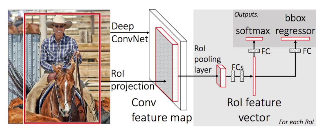
To accelerate R-CNN, Girshick (2015) redesigned the training procedure by merging three previously independent models into a single jointly trained framework, called Fast R-CNN. Rather than extracting CNN features separately for each region proposal, Fast R-CNN runs the CNN once over the full image to produce a feature map that is shared across all proposals. That shared feature map is then branched to support both object classification and bounding-box regression. In short, increased computation sharing is the main source of the speedup.
RoI Pooling
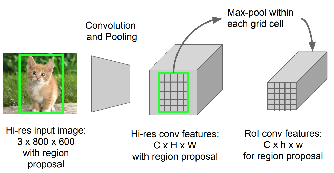
RoI pooling is a form of max pooling that converts features within a projected image region of arbitrary size, h x w, into a fixed-size output window, H x W. The input region is partitioned into H x W grids, with each subwindow approximately sized h/H x w/W. Max-pooling is then applied within each grid cell.
Model Workflow
The Fast R-CNN workflow can be outlined as follows; many steps match those in R-CNN:
- Pre-train a convolutional neural network on an image classification task.
- Generate region proposals using selective search (approximately 2k candidates per image).
- Modify the pre-trained CNN:
- Replace the final max pooling layer with a RoI pooling layer. RoI pooling produces fixed-length feature vectors for region proposals. Sharing CNN computation is especially beneficial because many proposals within the same image overlap heavily.
- Replace the final fully connected layer and the final softmax layer (K classes) with a fully connected layer and a softmax over K + 1 classes.
- Split the network into two output branches:
- A softmax estimator over K + 1 classes (as in R-CNN, with +1 for “background”), producing a discrete probability distribution per RoI.
- A bounding-box regression branch that predicts offsets relative to the original RoI for each of the K classes.
Loss Function
The model is trained with a loss that combines two tasks (classification + localization):
| Symbol | Explanation | | $u$ | True class label, $ u \in 0, 1, \dots, K$; by convention, the catch-all background class has $u = 0$. | | $p$ | Discrete probability distribution (per RoI) over K + 1 classes: $p = (p_0, \dots, p_K)$, computed by a softmax over the K + 1 outputs of a fully connected layer. | | $v$ | True bounding box $ v = (v_x, v_y, v_w, v_h) $. | | $t^u$ | Predicted bounding box correction, $t^u = (t^u_x, t^u_y, t^u_w, t^u_h)$. See above. | {:.info}
This loss adds the classification cost and the bounding box prediction cost: $\mathcal{L} = \mathcal{L}_\text{cls} + \mathcal{L}_\text{box}$. For a “background” RoI, $\mathcal{L}_\text{box}$ is excluded via the indicator function $\mathbb{1} [u \geq 1]$, defined as:
The full loss is:
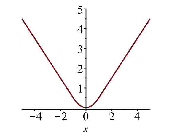
The bounding box loss $\mathcal{L}_{box}$ measures the discrepancy between $t^u_i$ and $v_i$ using a robust loss. Fast R-CNN uses the smooth L1 loss, which is described as being less sensitive to outliers.
Speed Bottleneck
Fast R-CNN significantly reduces training and inference time. However, the speed gains are limited because region proposals are still generated by a separate, computationally expensive algorithm.
Faster R-CNN
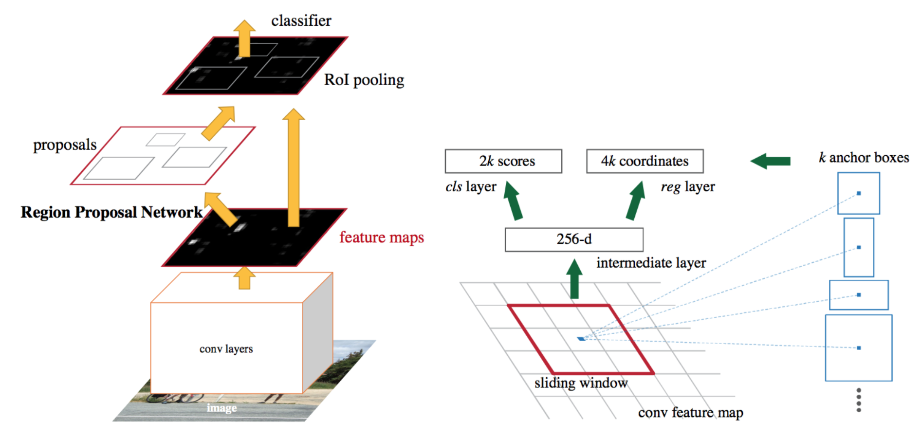
A straightforward way to further accelerate the pipeline is to incorporate region proposal generation into the CNN itself. Faster R-CNN (Ren et al., 2016) does exactly this by building a unified model that combines an RPN (region proposal network) with Fast R-CNN, sharing convolutional feature layers between them.
Model Workflow
- Pre-train a CNN network on image classification tasks.
- Fine-tune the RPN (region proposal network) end-to-end for the region proposal task, initialized from the pre-trained image classifier. Positive samples have IoU (intersection-over-union) > 0.7, while negative samples have IoU < 0.3.
- Slide a small n x n spatial window over the convolutional feature map of the full image.
- At the center of each sliding window, predict multiple regions with different scales and aspect ratios simultaneously. An anchor is defined by (sliding window center, scale, ratio). For example, 3 scales + 3 ratios => k=9 anchors at each sliding position.
- Train a Fast R-CNN object detector using proposals produced by the current RPN.
- Use the Fast R-CNN network to initialize RPN training. While keeping the shared convolutional layers fixed, fine-tune only the RPN-specific layers. At this point, the RPN and detection networks share convolutional layers.
- Fine-tune the Fast R-CNN specific layers.
- If needed, repeat Steps 4-5 to alternately train the RPN and Fast R-CNN.
Loss Function
Faster R-CNN is trained with a multi-task loss that is similar to the Fast R-CNN objective.
| Symbol | Explanation | | $p_i$ | Predicted probability of anchor i being an object. | | $p^*_i$ | Ground truth label (binary) of whether anchor i is an object. | | $t_i$ | Predicted four parameterized coordinates. | | $t^*_i$ | Ground truth coordinates. | | $N_\text{cls}$ | Normalization term, set to be mini-batch size (~256) in the paper. | | $N_\text{box}$ | Normalization term, set to the number of anchor locations (~2400) in the paper. | | $\lambda$ | A balancing parameter, set to be ~10 in the paper (so that both $\mathcal{L}_\text{cls}$ and $\mathcal{L}_\text{box}$ terms are roughly equally weighted). | {:.info}
The multi-task objective combines classification loss and bounding box regression loss:
where $\mathcal{L}_\text{cls}$ is the log loss over two classes. This formulation is equivalent to translating multi-class classification into a binary decision: whether the sample is a target object or not. $L_1^\text{smooth}$ is the smooth L1 loss.
Mask R-CNN
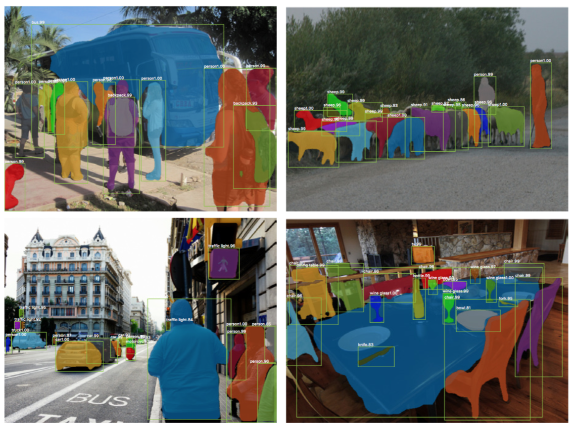
Mask R-CNN (He et al., 2017) extends Faster R-CNN to pixel-level image segmentation. The central idea is to decouple classification from pixel-level mask prediction. Building on Faster R-CNN, Mask R-CNN introduces a third branch that predicts an object mask in parallel with the existing classification and localization branches. The mask branch is a small fully-connected network applied to each RoI, producing a segmentation mask in a pixel-to-pixel fashion.
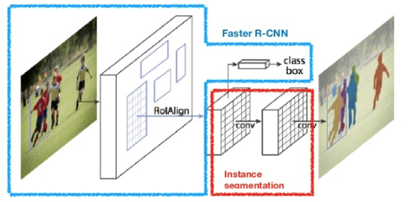
Because pixel-level segmentation requires finer alignment than bounding boxes, Mask R-CNN replaces RoI pooling with an improved layer called “RoIAlign,” enabling RoIs to be mapped onto the original image regions more accurately and precisely.
RoIAlign
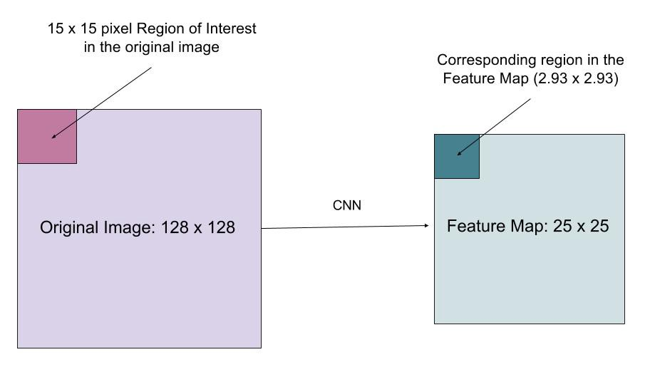
The RoIAlign layer addresses the spatial misalignment introduced by the quantization used in RoI pooling. RoIAlign removes the harsh quantization step, for example, by using x/16 rather than [x/16], so that extracted features align properly with the input pixels. Bilinear interpolation is used to compute feature values at floating-point locations in the input.
Loss Function
The Mask R-CNN multi-task loss combines classification, localization, and segmentation mask losses: $ \mathcal{L} = \mathcal{L}_\text{cls} + \mathcal{L}_\text{box} + \mathcal{L}_\text{mask}$, where $\mathcal{L}_\text{cls}$ and $\mathcal{L}_\text{box}$ are the same as in Faster R-CNN.
The mask branch outputs a mask of size m x m for each RoI and for each class (K classes total). Therefore, the full output has size $K \cdot m^2$. Since the model learns one mask per class, mask generation does not involve competition among classes.
$\mathcal{L}_\text{mask}$ is defined as the mean binary cross-entropy loss, including only the k-th mask when the region corresponds to ground truth class k.
where $y_{ij}$ is the label of cell (i, j) in the ground-truth mask for the m x m region, and $\hat{y}_{ij}^k$ is the predicted value at the same cell in the mask learned for the ground-truth class k.
Summary of Models in the R-CNN family
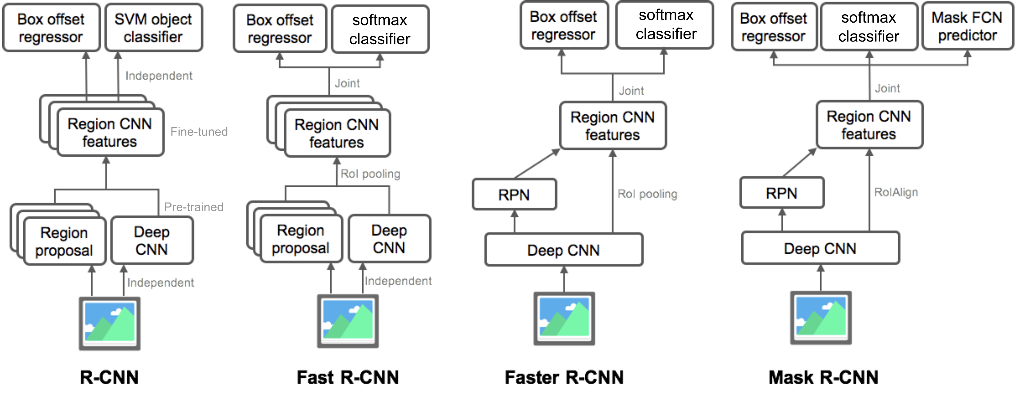
Below is an illustration of the designs of R-CNN, Fast R-CNN, Faster R-CNN, and Mask R-CNN. By comparing the small changes between diagrams, you can see how each model evolves into the next.
Cited as:
@article{weng2017detection3,
  title   = "Object Detection for Dummies Part 3: R-CNN Family",
  author  = "Weng, Lilian",
  journal = "lilianweng.github.io",
  year    = "2017",
  url     = "https://lilianweng.github.io/posts/2017-12-31-object-recognition-part-3/"
}
Reference
[1] Ross Girshick, Jeff Donahue, Trevor Darrell, and Jitendra Malik. “Rich feature hierarchies for accurate object detection and semantic segmentation.” In Proc. IEEE Conf. on computer vision and pattern recognition (CVPR), pp. 580-587. 2014.
[2] Ross Girshick. “Fast R-CNN.” In Proc. IEEE Intl. Conf. on computer vision, pp. 1440-1448. 2015.
[3] Shaoqing Ren, Kaiming He, Ross Girshick, and Jian Sun. “Faster R-CNN: Towards real-time object detection with region proposal networks.” In Advances in neural information processing systems (NIPS), pp. 91-99. 2015.
[4] Kaiming He, Georgia Gkioxari, Piotr Dollár, and Ross Girshick. “Mask R-CNN.” arXiv preprint arXiv:1703.06870, 2017.
[5] Joseph Redmon, Santosh Divvala, Ross Girshick, and Ali Farhadi. “You only look once: Unified, real-time object detection.” In Proc. IEEE Conf. on computer vision and pattern recognition (CVPR), pp. 779-788. 2016.
[6] “A Brief History of CNNs in Image Segmentation: From R-CNN to Mask R-CNN” by Athelas.
[7] Smooth L1 Loss: https://github.com/rbgirshick/py-faster-rcnn/files/764206/SmoothL1Loss.1.pdf