In Part 3, we reviewed models in the R-CNN family. Those methods are region-based object detection algorithms. Although they can deliver high accuracy, they may be too slow for some use cases, such as autonomous driving. Part 4 focuses exclusively on fast object detection models, including SSD, RetinaNet, and models in the YOLO family.

Links to all posts in the series: [Part 1] [Part 2] [Part 3] [Part 4].

Two-stage vs One-stage Detectors

All models in the R-CNN family are region-based. Detection is carried out in two stages: (1) the model first proposes a set of regions of interest via selective search or a region proposal network. These proposals are sparse because the space of potential bounding boxes is effectively unbounded. (2) A classifier then processes only the proposed region candidates.

The alternative approach skips region proposals and runs detection directly over a dense sampling of possible locations. This is the defining behavior of a one-stage object detection algorithm. The design is faster and simpler, but it can reduce performance somewhat.

All models discussed in this post are one-stage detectors.

YOLO: You Only Look Once

The YOLO model (“You Only Look Once”; Redmon et al., 2016) was the first major attempt to build a fast, real-time object detector. Because YOLO avoids the region proposal step and predicts only a limited set of bounding boxes, it can run inference very quickly.

Workflow

1. Pre-train a CNN on an image classification task.

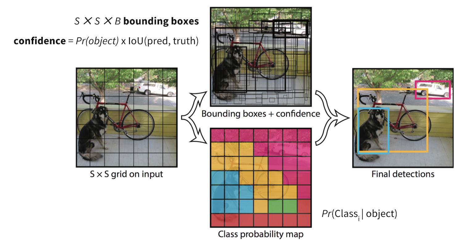
2. Split an image into $S \times S$ cells. If an object’s center lies within a cell, that cell becomes “responsible” for predicting that object. Each cell predicts: (a) the locations of $B$ bounding boxes, (b) a confidence score, and (c) a probability distribution over object classes, conditioned on an object being present in the bounding box.

   • The bounding box coordinates are represented by a 4-tuple (center x-coord, center y-coord, width, height), $(x, y, w, h)$, where $x$ and $y$ are defined as offsets relative to the cell location. In addition, $x$, $y$, $w$, and $h$ are normalized by the image width and height, so they lie within (0, 1].
   • A confidence score reflects how likely it is that the cell contains an object: Pr(containing an object) x IoU(pred, truth); where Pr = probability and IoU = interaction under union.
   • If the cell contains an object, it predicts a probability that the object belongs to each class $C_i, i=1, \dots, K$: Pr(the object belongs to the class C_i | containing an object). At this step, the model outputs only one set of class probabilities per cell, independent of the number of bounding boxes, $B$.
   • Overall, one image contains $S \times S \times B$ bounding boxes. Each box contributes 4 location predictions, 1 confidence score, and K conditional class probabilities. The total number of prediction values for one image is $S \times S \times (5B + K)$, which matches the tensor shape of the model’s final convolutional layer.

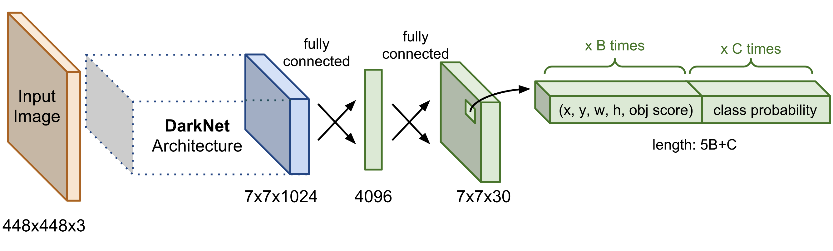
3. The last layer of the pre-trained CNN is replaced so that it outputs a prediction tensor of size $S \times S \times (5B + K)$.

Network Architecture

The base network is similar to GoogLeNet, except the inception modules are replaced with 1x1 and 3x3 convolutional layers. The final prediction, with shape $S \times S \times (5B + K)$, is generated by two fully connected layers applied over the full convolutional feature map.

Loss Function

The loss has two components: a localization loss for bounding box offset prediction and a classification loss for conditional class probabilities. Both are computed using sums of squared errors. Two scaling factors control the relative weighting: one increases the loss from bounding box coordinate predictions ($\lambda_\text{coord}$), and the other decreases the loss contribution from confidence score predictions for boxes that do not contain objects ($\lambda_\text{noobj}$). Reducing the background-box contribution is important because most predicted boxes correspond to no object. In the paper, the model uses $\lambda_\text{coord} = 5$ and $\lambda_\text{noobj} = 0.5$.

NOTE: In the original YOLO paper, the loss function uses $C_i$ instead of $C_{ij}$ as confidence score. I made the correction based on my own understanding, since every bounding box should have its own confidence score. Please kindly let me if you do not agree. Many thanks.

where,

• $\mathbb{1}_i^\text{obj}$: An indicator function for whether cell i contains an object.
• $\mathbb{1}_{ij}^\text{obj}$: An indicator for whether the j-th bounding box in cell i is “responsible” for predicting the object (see Fig. 3).
• $C_{ij}$: The confidence score for cell i, Pr(containing an object) * IoU(pred, truth).
• $\hat{C}_{ij}$: The predicted confidence score.
• $\mathcal{C}$: The set of all classes.
• $p_i(c)$: The conditional probability that cell i contains an object of class $c \in \mathcal{C}$.
• $\hat{p}_i(c)$: The predicted conditional class probability.

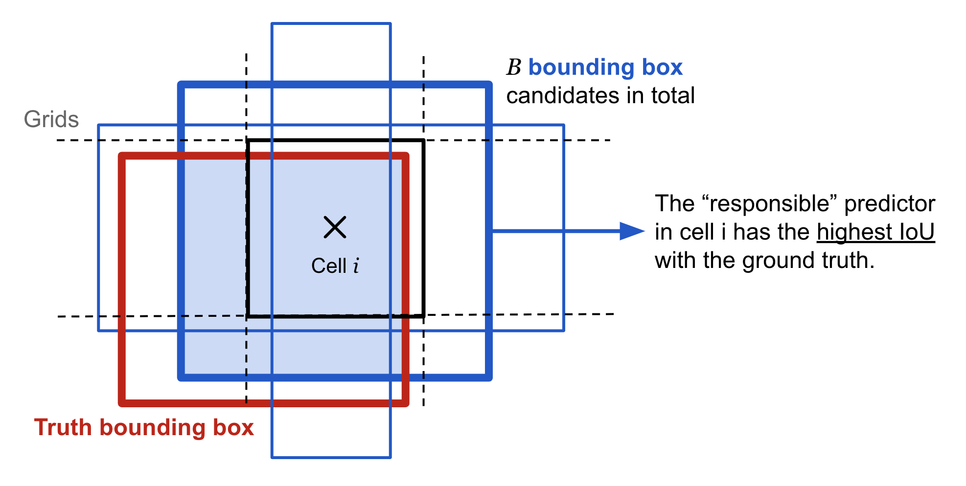
The loss penalizes classification error only when an object exists in the corresponding grid cell, $\mathbb{1}_i^\text{obj} = 1$. It also penalizes bounding box coordinate error only when the predictor is “responsible” for the ground-truth box, $\mathbb{1}_{ij}^\text{obj} = 1$.

As a one-stage detector, YOLO is very fast, but it performs poorly on irregularly shaped objects or groups of small objects, due to the limited number of bounding box candidates.

SSD: Single Shot MultiBox Detector

The Single Shot Detector (SSD; Liu et al, 2016) was one of the first approaches to leverage a convolutional neural network’s pyramidal feature hierarchy to efficiently detect objects across a wide range of sizes.

Image Pyramid

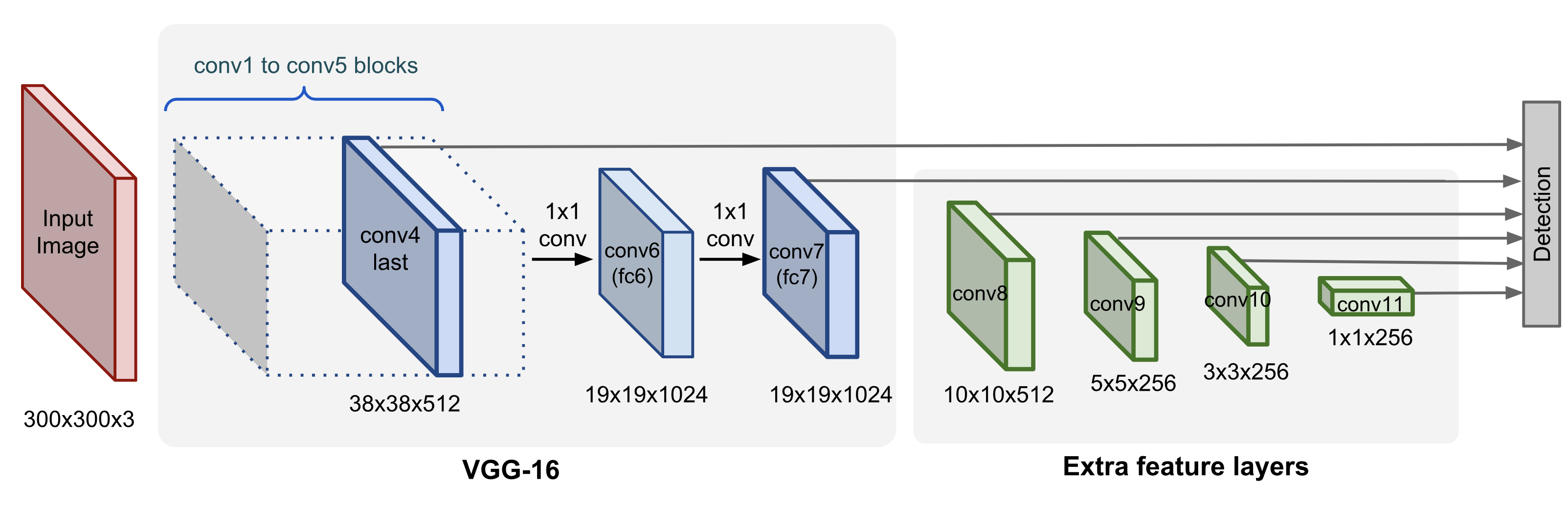
SSD uses the VGG-16 model, pre-trained on ImageNet, as its backbone for extracting image features. On top of VGG16, SSD appends several convolutional feature layers with progressively smaller spatial dimensions. Together, these layers form a pyramid representation at multiple scales. Intuitively, earlier levels with larger, fine-grained feature maps are well suited to small objects, while later levels with smaller, coarse-grained maps are effective for large objects. In SSD, detection is performed at every pyramid layer so that each layer specializes in objects at different scales.

Workflow

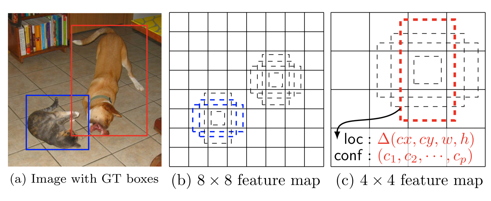
Unlike YOLO, SSD does not partition the image into arbitrary grids. Instead, it predicts offsets relative to predefined anchor boxes (called “default boxes” in the paper) at every location in each feature map. Each anchor box has a fixed size and position relative to its associated feature cell. These anchor boxes tile the feature map in a convolutional fashion.

Feature maps at different pyramid levels have different receptive-field sizes. SSD rescales anchor boxes across levels so that each feature map is responsible for objects at a particular scale. For example, in Fig. 5, the dog is detectable only on the 4x4 feature map (a higher level), while the cat is captured on the 8x8 feature map (a lower level).

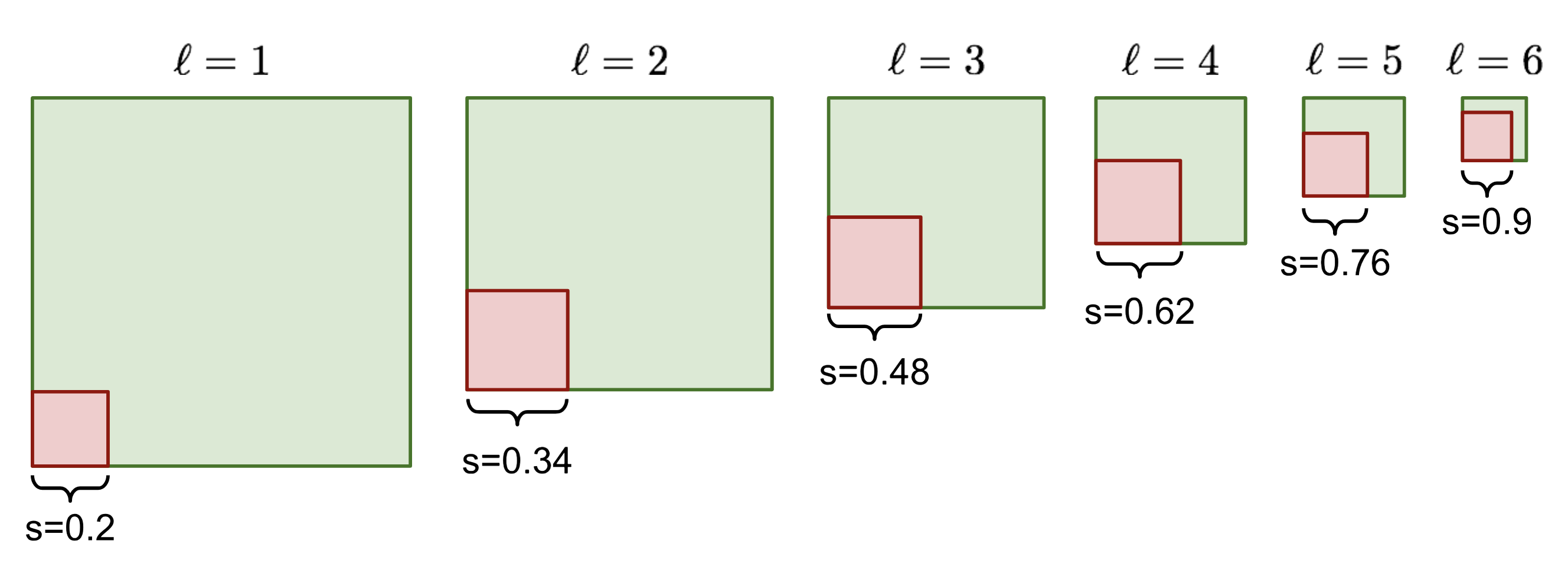
The width, height, and center coordinates of an anchor box are all normalized to (0, 1). At a location $(i, j)$ in the $\ell$-th feature layer with size $m \times n$, $i=1,\dots,n, j=1,\dots,m$, a unique linear scale is defined (proportional to the layer level), along with 5 different box aspect ratios (width-to-height ratios). Additionally, there is a special scale (the paper does not explain why; possibly a heuristic) when the aspect ratio is 1. This yields 6 anchor boxes per feature cell.

At every spatial location, the model outputs 4 offsets and $c$ class probabilities by applying a $3 \times 3 \times p$ convolutional filter (where $p$ is the number of channels in the feature map) for each of the $k$ anchor boxes. Therefore, for a feature map of size $m \times n$, the model requires $kmn(c+4)$ prediction filters.

Loss Function

As in YOLO, SSD uses a loss that combines localization loss and classification loss.

$\mathcal{L} = \frac{1}{N}(\mathcal{L}_\text{cls} + \alpha \mathcal{L}_\text{loc})$

where $N$ is the number of matched bounding boxes and $\alpha$ balances the two loss terms, selected via cross validation.

The localization loss is a smooth L1 loss between the predicted bounding-box corrections and the true values. The coordinate correction transformation is the same as what R-CNN uses in bounding box regression.

where $\mathbb{1}_{ij}^\text{match}$ indicates whether the $i$-th bounding box, with coordinates $(p^i_x, p^i_y, p^i_w, p^i_h)$, is matched to the $j$-th ground-truth box, with coordinates $(g^j_x, g^j_y, g^j_w, g^j_h)$, for any object. $d^i_m, m\in\{x, y, w, h\}$ are the predicted correction terms. See this for details on how the transformation works.

The classification loss is a softmax loss over multiple classes (softmax_cross_entropy_with_logits in tensorflow):

where $\mathbb{1}_{ij}^k$ indicates whether the $i$-th bounding box and the $j$-th ground-truth box are matched for an object in class $k$. $\text{pos}$ is the set of matched bounding boxes ($N$ items total), and $\text{neg}$ is the set of negative examples. SSD applies hard negative mining to choose easily misclassified negative examples for the $\text{neg}$ set: after sorting all anchor boxes by objectiveness confidence score, the model selects top candidates for training so that the neg:pos ratio is at most 3:1.

YOLOv2 / YOLO9000

YOLOv2 (Redmon & Farhadi, 2017) is an improved version of YOLO. YOLO9000 extends YOLOv2 and is trained jointly on a combined dataset that merges the COCO detection dataset with the top 9000 classes from ImageNet.

YOLOv2 Improvement

YOLOv2 introduces multiple changes aimed at improving accuracy while maintaining speed, including:

1. BatchNorm helps: Batch normalization is added to all convolutional layers, yielding a substantial improvement in convergence.

2. Image resolution matters: Fine-tuning the base model on high resolution images improves detection quality.

3. Convolutional anchor box detection: Instead of predicting bounding box coordinates using fully connected layers over the full feature map, YOLOv2 uses convolutional layers to predict anchor boxes, similar to Faster R-CNN. Spatial localization and class probability prediction are separated. Overall, this change slightly reduces mAP but increases recall.

4. K-mean clustering of box dimensions: Unlike Faster R-CNN, which uses hand-selected anchor box sizes, YOLOv2 applies k-mean clustering on training data to derive effective priors for anchor box dimensions. The distance metric is designed to depend on IoU:

where $x$ is a ground-truth box candidate and $c_i$ is a centroid. The best number of centroids (anchor boxes), $k$, can be selected using the elbow method.

Anchor boxes obtained from clustering achieve better average IoU for a fixed number of boxes.

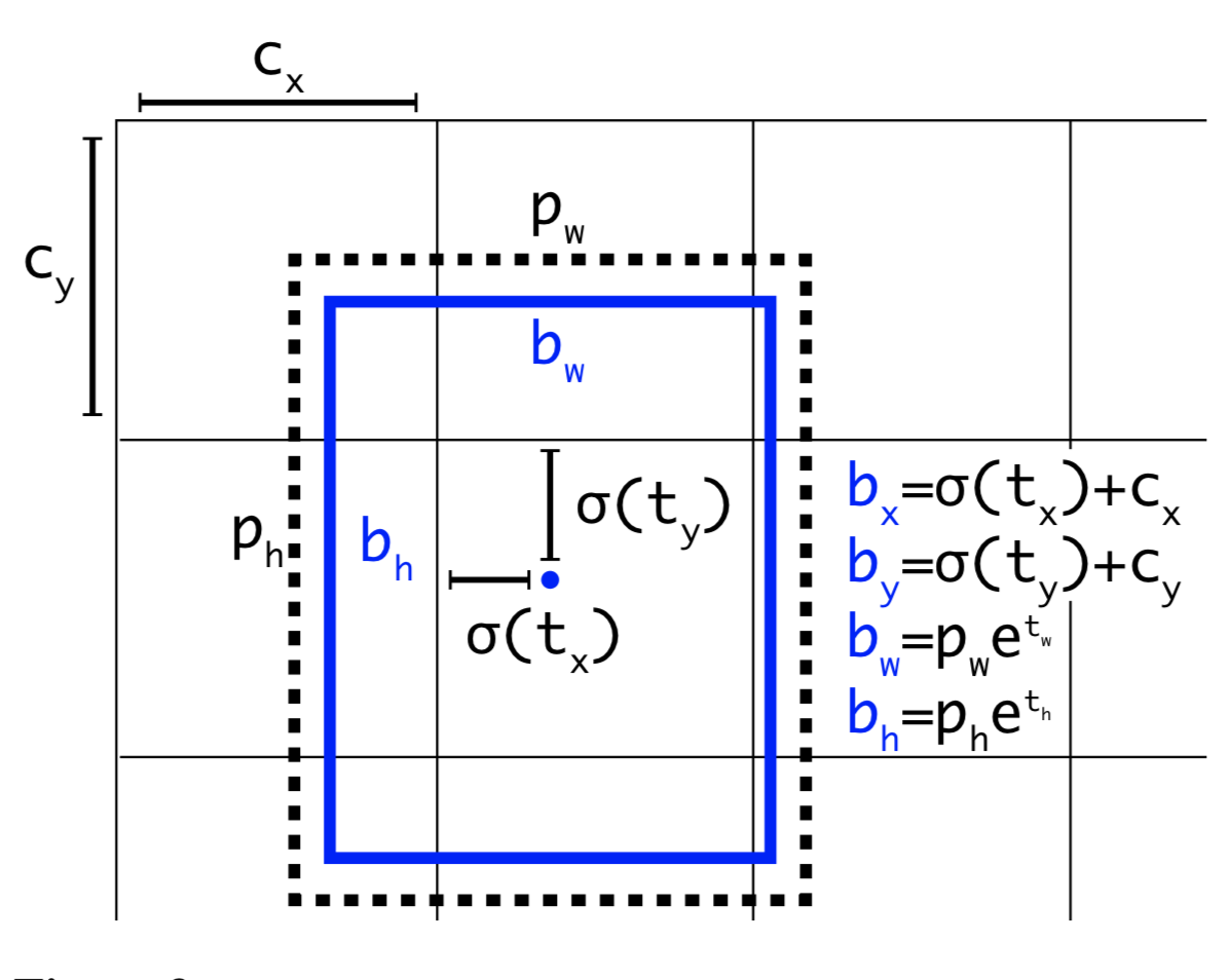
5. Direct location prediction: YOLOv2 restructures bounding box prediction to prevent divergence from the cell center. If predictions are allowed to place a box anywhere in the image (as in a region proposal network), training can become unstable.

Given an anchor box of size $(p_w, p_h)$ at a grid cell whose top-left corner is $(c_x, c_y)$, the model predicts offsets and scales, $(t_x, t_y, t_w, t_h)$. The resulting predicted bounding box $b$ has center $(b_x, b_y)$ and size $(b_w, b_h)$. The confidence score is computed as sigmoid ($\sigma$) of an output term $t_o$.

6. Add fine-grained features: YOLOv2 introduces a passthrough layer that brings fine-grained features from an earlier layer into the final output layer. This passthrough mechanism is similar to identity mappings in ResNet, enabling extraction of higher-dimensional features from earlier layers. This change improves performance by 1%.

7. Multi-scale training: To make the model robust to varied input sizes, a new input dimension is randomly sampled every 10 batches. Because YOLOv2 convolutional layers downsample by a factor of 32, the sampled size is always a multiple of 32.

8. Light-weighted base model: To further accelerate prediction, YOLOv2 uses a lightweight backbone, DarkNet-19, which includes 19 convolutional layers and 5 max-pooling layers. A key design choice is inserting average pooling and 1x1 convolutional filters between 3x3 convolutional layers.

YOLO9000: Rich Dataset Training

Because annotating bounding boxes for detection is far more expensive than assigning classification labels, the paper proposes combining a small detection dataset with a large classification dataset (ImageNet) so that the model can be trained across many more object categories. The name YOLO9000 refers to the top 9000 classes in ImageNet. During joint training, when an input image comes from the classification dataset, the model backpropagates only the classification loss.

The detection dataset uses fewer and more general labels. In addition, labels across datasets are often not mutually exclusive. For example, ImageNet may label an image as “Persian cat,” while COCO would label the same image as “cat.” Without mutual exclusivity, applying a single softmax across all classes is not appropriate.

To merge ImageNet labels (1000 classes, fine-grained) with COCO/PASCAL labels (< 100 classes, coarse-grained) efficiently, YOLO9000 constructs a hierarchical tree guided by WordNet, placing general labels closer to the root and fine-grained labels at the leaves. Under this structure, “cat” becomes the parent node of “Persian cat.”

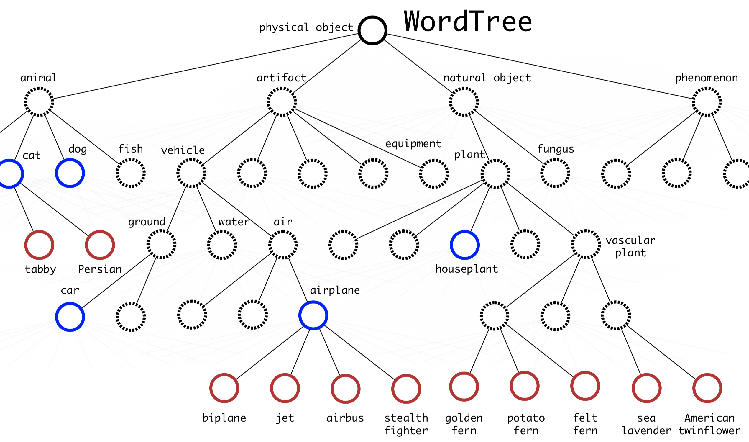
To compute the probability for a given class node, follow the path from that node up to the root:

Pr("persian cat" | contain a "physical object") 
= Pr("persian cat" | "cat") 
  Pr("cat" | "animal") 
  Pr("animal" | "physical object") 
  Pr(contain a "physical object")    # confidence score.

Note that Pr(contain a "physical object") is the confidence score, which is predicted separately in the bounding box detection pipeline. The conditional-probability chain can terminate at any step, depending on which labels are available.

RetinaNet

RetinaNet (Lin et al., 2018) is a one-stage dense object detector. It relies on two key components: a featurized image pyramid and focal loss.

Focal Loss

A major challenge in training object detection models is the extreme class imbalance between background regions (no objects) and foreground regions (objects of interest). Focal loss addresses this by assigning higher weight to hard, easily misclassified examples (for example, background with noisy texture or partial objects) and reducing the weight for easy examples (for example, clearly empty background).

Starting from the standard cross-entropy loss for binary classification,

where $y \in \{0, 1\}$ is the binary ground-truth label indicating whether a bounding box contains an object, and $p \in [0, 1]$ is the predicted probability of objectiveness (that is, the confidence score).

For notational convenience,

Easy examples with large $p_t \gg 0.5$, meaning $p$ is close to 0 (when y=0) or close to 1 (when y=1), can still produce a loss of non-trivial magnitude. Focal loss explicitly multiplies each cross-entropy term by a weighting factor $(1-p_t)^\gamma, \gamma \geq 0$, such that the weight becomes small when $p_t$ is large, thereby down-weighting easy examples.

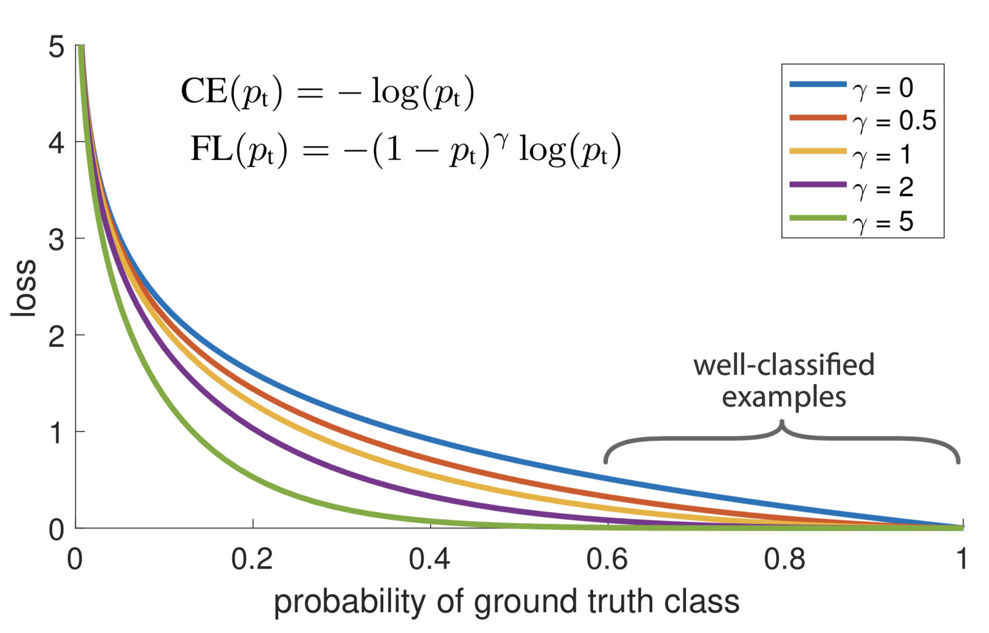
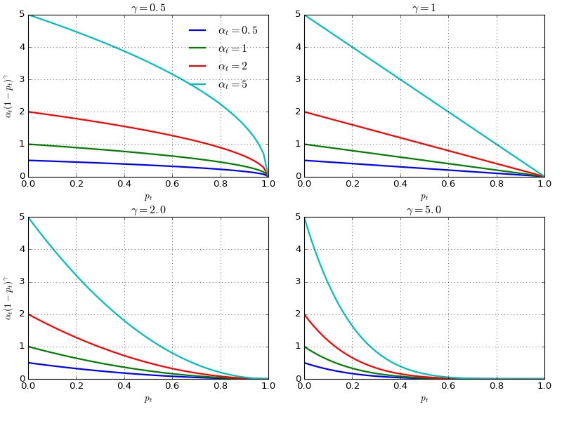
To better control the shape of the weighting function (see Fig. 10.), RetinaNet uses an $\alpha$-balanced variant of focal loss, where $\alpha=0.25, \gamma=2$ performs best.

Featurized Image Pyramid

The featurized image pyramid (Lin et al., 2017) serves as the backbone network for RetinaNet. Similar to the image pyramid approach used in SSD, featurized image pyramids provide a standard vision component for multi-scale object detection.

The central idea of the feature pyramid network is illustrated in the base design: it consists of a sequence of pyramid levels, each aligned with a network stage. A stage contains multiple convolutional layers of the same spatial size, and stage sizes are downsampled by a factor of 2 between adjacent stages. Let the final layer of the $i$-th stage be $C_i$.

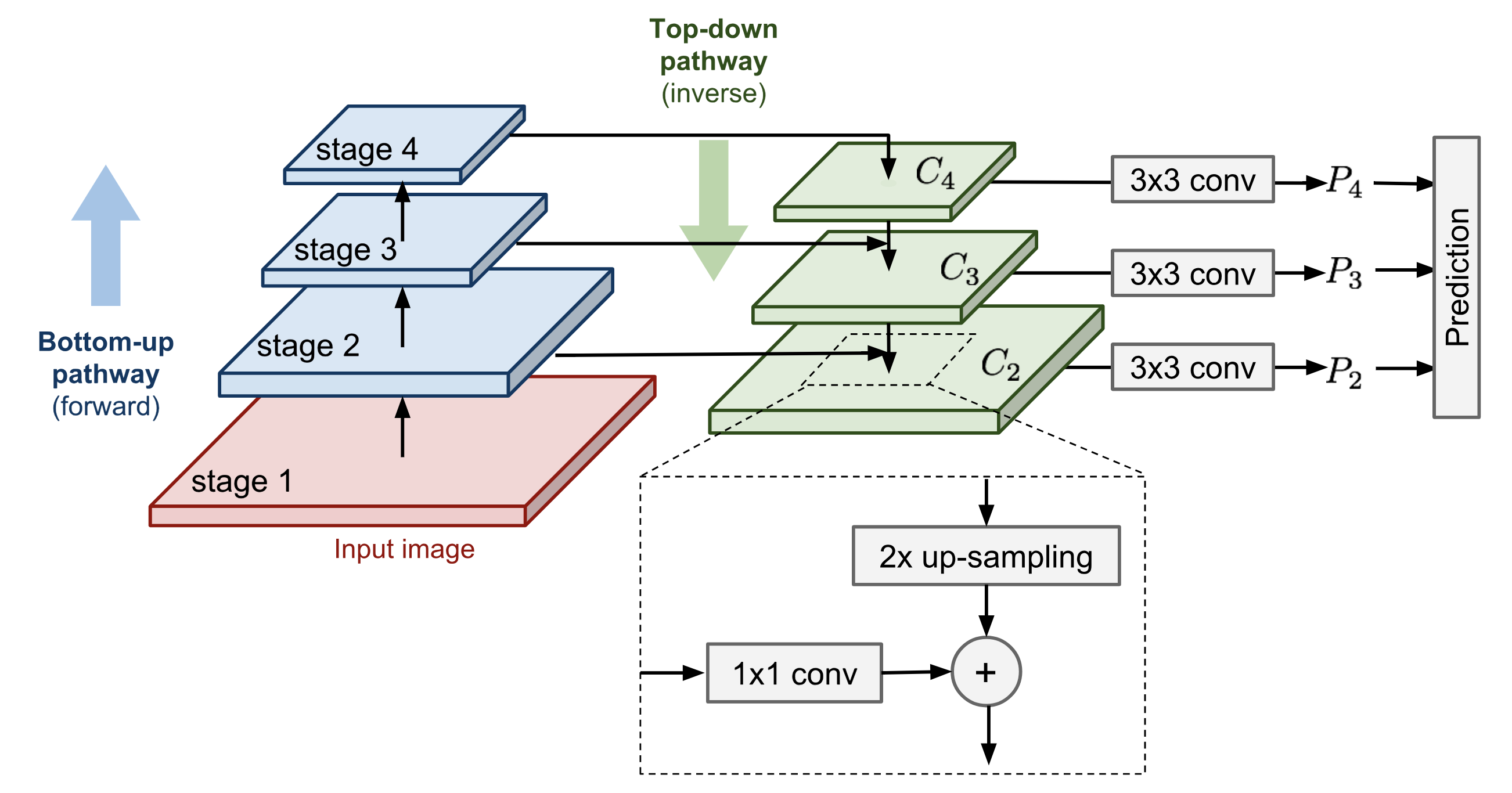
Two pathways connect convolutional layers:

• Bottom-up pathway: the standard feedforward computation path.
• Top-down pathway: the reverse-direction pathway that injects coarse but semantically stronger feature maps into earlier pyramid levels (which have larger spatial resolution) using lateral connections.
  • First, higher-level features are upsampled spatially so the map becomes 2x larger. The paper uses nearest-neighbor upsampling. While many image upscaling algorithms exist (for example, deconv), using a different scaling method may or may not improve RetinaNet performance.
  • The upsampled feature map is passed through a 1x1 convolution to reduce the channel dimension.
  • Finally, the two feature maps are merged via element-wise addition.
    
    Lateral connections are applied only at the final layer of each stage, denoted as $\{C_i\}$, and the procedure continues until the finest (largest) merged feature map is produced. Predictions are generated from every merged map after a 3x3 convolution, $\{P_i\}$.

Ablation studies indicate the following importance ranking for components of the featurized image pyramid design: 1x1 lateral connection > detecting objects across multiple layers > top-down enrichment > pyramid representation (relative to checking only the finest layer).

Model Architecture

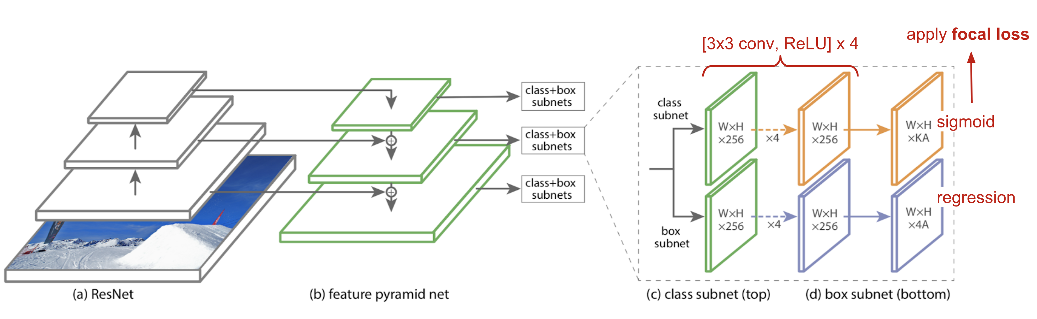
The featurized pyramid is built on top of the ResNet architecture. Recall that ResNet contains 5 convolutional blocks (that is, network stages or pyramid levels). The final layer of the $i$-th pyramid level, $C_i$, has a resolution that is $2^i$ lower than the raw input dimensions.

RetinaNet uses feature pyramid levels $P_3$ through $P_7$:

• $P_3$ through $P_5$ are computed from the corresponding ResNet residual stages $C_3$ through $C_5$. These levels are linked via both top-down and bottom-up pathways.
• $P_6$ is produced by applying a 3×3 stride-2 convolution on top of $C_5$.
• $P_7$ applies ReLU followed by a 3×3 stride-2 convolution on $P_6$.

Extending ResNet with higher pyramid levels improves performance when detecting large objects.

As in SSD, detection is performed at all pyramid levels by generating predictions from each merged feature map. Because these predictions share the same classifier and box regressor, they are all constrained to the same channel dimension, d=256.

Each level contains A=9 anchor boxes:

• The base sizes correspond to areas of $32^2$ through $512^2$ pixels on $P_3$ through $P_7$, respectively. Three size ratios are used, $\{2^0, 2^{1/3}, 2^{2/3}\}$.
• For each size, three aspect ratios are used: {1/2, 1, 2}.

As usual, for each anchor box the model outputs (1) a class probability for each of $K$ classes in the classification subnet and (2) a regressed offset from the anchor box to the nearest ground-truth object in the box regression subnet. The classification subnet uses the focal loss introduced above.

YOLOv3

YOLOv3 is developed by applying a collection of design tricks to YOLOv2. These changes are motivated by recent advances in object detection.

The changes are as follows:

1. Logistic regression for confidence scores: YOLOv3 predicts a confidence score for each bounding box using logistic regression, whereas YOLO and YOLOv2 use a sum of squared errors for classification terms (see the loss function above). Using linear regression for offset prediction leads to reduced mAP.

2. No more softmax for class prediction: For class confidence prediction, YOLOv3 uses multiple independent logistic classifier for each class instead of a single softmax layer. This is particularly beneficial because an image may contain multiple labels, and the labels are not necessarily mutually exclusive.

3. Darknet + ResNet as the base model: The updated Darknet-53 continues to rely on successive 3x3 and 1x1 convolution layers, similar to the original dark net architecture, but adds residual blocks.

4. Multi-scale prediction: Inspired by image pyramids, YOLOv3 adds several convolution layers after the base feature extractor and produces predictions at three different scales across these layers. As a result, it evaluates many more bounding box candidates spanning a wide range of sizes.

5. Skip-layer concatenation: YOLOv3 also introduces cross-layer connections between two prediction layers (excluding the output layer) and earlier, finer-grained feature maps. The model first up-samples the coarse feature maps and then merges them with earlier features via concatenation. Incorporating finer-grained information improves small-object detection.

Notably, focal loss does not benefit YOLOv3, potentially due to the use of $\lambda_\text{noobj}$ and $\lambda_\text{coord}$, which increase the loss from bounding box location predictions and decrease the loss from confidence predictions for background boxes.

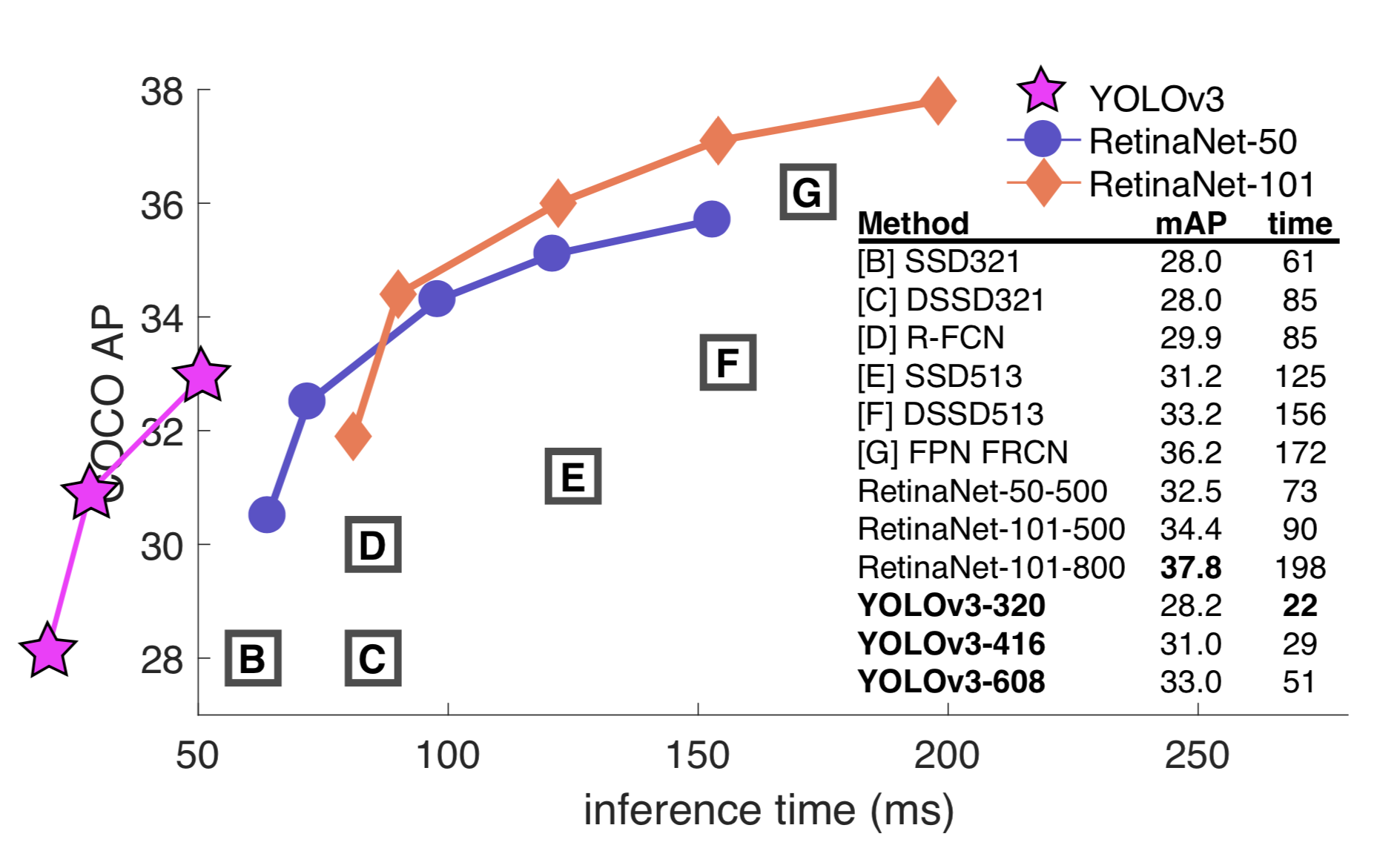
Overall, YOLOv3 is faster and performs better than SSD, and it performs worse than RetinaNet but is 3.8x faster.

Cited as:

@article{weng2018detection4,
  title   = "Object Detection Part 4: Fast Detection Models",
  author  = "Weng, Lilian",
  journal = "lilianweng.github.io",
  year    = "2018",
  url     = "https://lilianweng.github.io/posts/2018-12-27-object-recognition-part-4/"
}

Reference

[1] Joseph Redmon, et al. “You only look once: Unified, real-time object detection.” CVPR 2016.

[2] Joseph Redmon and Ali Farhadi. “YOLO9000: Better, Faster, Stronger.” CVPR 2017.

[3] Joseph Redmon, Ali Farhadi. “YOLOv3: An incremental improvement.”.

[4] Wei Liu et al. “SSD: Single Shot MultiBox Detector.” ECCV 2016.

[5] Tsung-Yi Lin, et al. “Feature Pyramid Networks for Object Detection.” CVPR 2017.

[6] Tsung-Yi Lin, et al. “Focal Loss for Dense Object Detection.” IEEE transactions on pattern analysis and machine intelligence, 2018.

[7] “What’s new in YOLO v3?” by Ayoosh Kathuria on “Towards Data Science”, Apr 23, 2018.