Attention: Attention!
[Updated on 2018-10-28: Added Pointer Network and a link to my Transformer implementation.] [Updated on 2018-11-06: Added a link to the Transformer model implementation.] [Updated on 2018-11-18: Added Neural Turing Machines.] [Updated on 2019-07-18: Corrected an error involving the use of the term “self-attention” when introducing the show-attention-tell paper, and moved that content to the Self-Attention section.] [Updated on 2020-04-07: A follow-up post on improved Transformer models is here.]
· 21 min read · Curated and presented by Arthur Sedek
[Updated on 2018-10-28: Add Pointer Network and the link to my implementation of Transformer.]
[Updated on 2018-11-06: Add a link to the implementation of Transformer model.]
[Updated on 2018-11-18: Add Neural Turing Machines.]
[Updated on 2019-07-18: Correct the mistake on using the term “self-attention” when introducing the show-attention-tell paper; moved it to Self-Attention section.]
[Updated on 2020-04-07: A follow-up post on improved Transformer models is here.]
To a certain extent, attention is inspired by how humans allocate visual focus across different regions of an image, as well as by how we relate words within a sentence or across nearby context. Consider the Shiba Inu photo in Fig. 1.

Human visual attention lets us concentrate on a specific region with “high resolution” (for example, the pointy ear inside the yellow box) while still perceiving the surrounding content in “low resolution” (for instance, the snowy background and the outfit). We then shift the focal point or draw inferences accordingly. When given a small image patch, pixels elsewhere in the scene provide cues about what should appear in that patch. We anticipate a pointy ear in the yellow box because we can already observe a dog’s nose, another pointy ear on the right, and the Shiba’s characteristic eyes (elements in the red boxes). In contrast, the sweater and blanket at the bottom offer much weaker evidence than those dog-specific features.
In the same spirit, we can describe relationships among words within a sentence or within a short context window. When we encounter “eating”, we typically expect a food-related word to appear soon. A color adjective may describe that food, but it is often less directly related to “eating” itself.
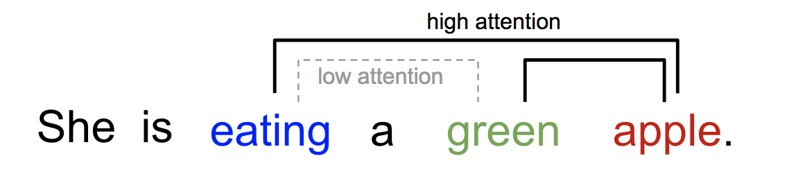
In short, attention in deep learning can be interpreted as a vector of importance weights. To predict or infer one element, such as a pixel in an image or a word in a sentence, we use an attention vector to estimate how strongly that element is correlated with (or “attends to”, as commonly phrased in the literature) other elements. We then approximate the target by taking a weighted sum of those other elements’ values, using the attention vector as weights.
What’s Wrong with Seq2Seq Model?
The seq2seq model originated in language modeling (Sutskever, et al. 2014). At a high level, it seeks to map an input sequence (the source) to an output sequence (the target), where both sequences may have arbitrary lengths. Typical transformations include machine translation across languages (in text or audio form), question-answer dialog generation, and even converting sentences into grammar trees.
Seq2seq models commonly use an encoder-decoder architecture consisting of the following components:
- An encoder that processes the input sequence and compresses the information into a context vector (also called a sentence embedding or “thought” vector) of fixed length. This representation is intended to summarize the meaning of the entire source sequence.
- A decoder that is initialized from the context vector and generates the transformed output. Early approaches used only the encoder’s final state as the decoder’s initial state.
Both the encoder and decoder are recurrent neural networks, typically built with LSTM or GRU units.
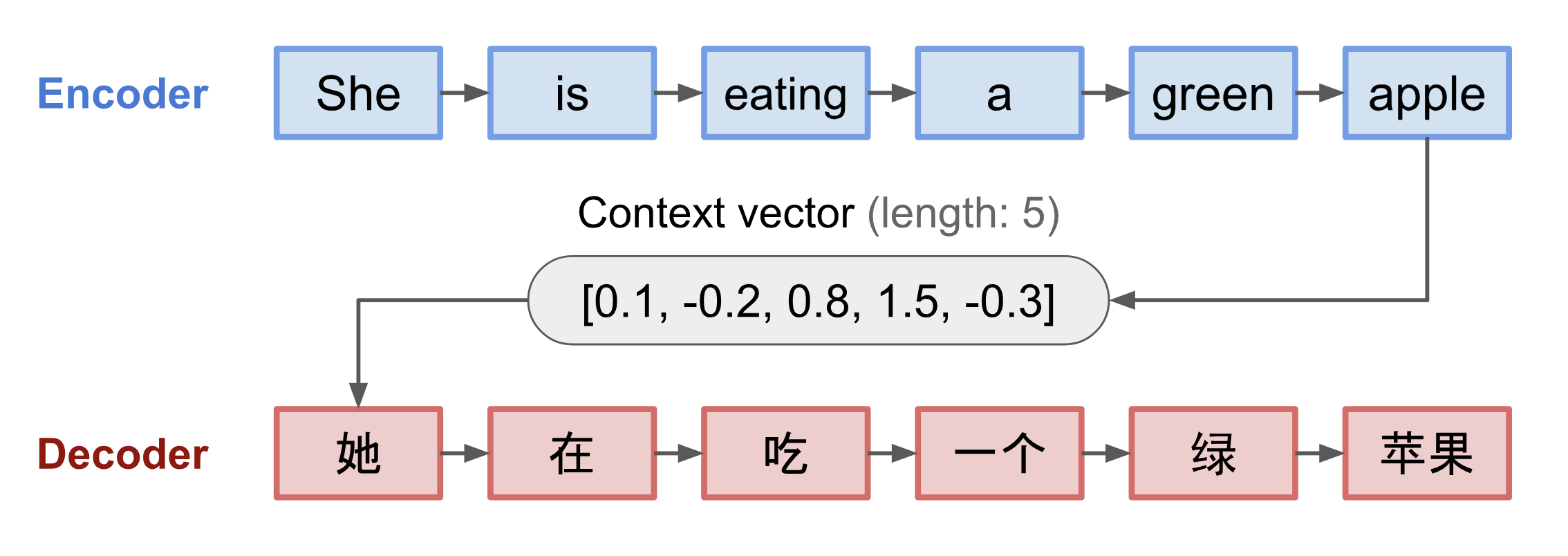
A key and well-known limitation of using a fixed-length context vector is that it struggles to retain information from long sentences. In practice, by the time the model finishes processing the full input, it often has effectively “forgotten” the beginning. The attention mechanism was introduced (Bahdanau et al., 2015) to address this issue.
Born for Translation
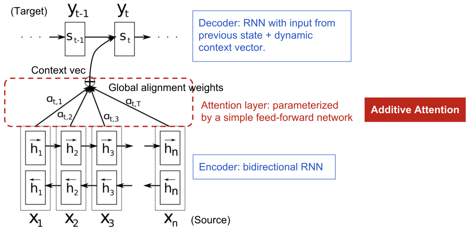
Attention was introduced to improve the ability to remember long source sentences in neural machine translation (NMT). Instead of constructing a single context vector solely from the encoder’s final hidden state, the central innovation of attention is to create shortcut connections between the context vector and the entire source input. Importantly, the weights on these shortcut connections can differ for each output element.
Because the context vector can reference the whole input sequence, the model no longer needs to rely on a single compressed summary that can be overwritten or forgotten. The source-target alignment is learned and managed through the context vector. Concretely, the context vector incorporates three types of information:
- encoder hidden states;
- decoder hidden states;
- alignment between source and target.
Definition
Next, we define the attention mechanism introduced for NMT in a more formal way. Suppose we have a source sequence $\mathbf{x}$ of length $n$ and we aim to produce a target sequence $\mathbf{y}$ of length $m$:
(Boldface variables indicate vectors, and the same convention applies throughout this post.)
The encoder is a bidirectional RNN (or another recurrent configuration of your choice) with a forward hidden state $\overrightarrow{\boldsymbol{h}}_i$ and a backward hidden state $\overleftarrow{\boldsymbol{h}}_i$. The encoder state is represented by a simple concatenation of the two, motivated by the desire to annotate each word using information from both preceding and following words.
The decoder has hidden state $\boldsymbol{s}_t=f(\boldsymbol{s}_{t-1}, y_{t-1}, \mathbf{c}_t)$ for the output word at position t, $t=1,\dots,m$. The context vector $\mathbf{c}_t$ is defined as a weighted sum over the input sequence hidden states, where the weights are determined by alignment scores:
The alignment model assigns a score $\alpha_{t,i}$ to the pair consisting of the input at position i and the output at position t, $(y_t, x_i)$, reflecting how well they match. The set of $\{\alpha_{t, i}\}$ forms weights that determine how much each source hidden state contributes to each output. In Bahdanau’s work, the alignment score $\alpha$ is parameterized by a feed-forward network with a single hidden layer, and this network is trained jointly with the rest of the model. Using tanh as the non-linear activation, the score function takes the following form:
where $\mathbf{v}_a$ and $\mathbf{W}_a$ are weight matrices learned by the alignment model.
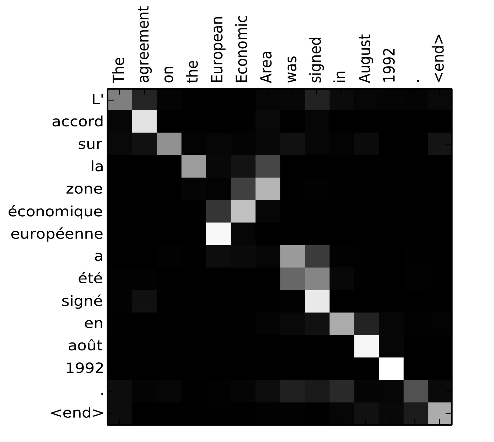
The resulting alignment score matrix is a useful byproduct, because it explicitly visualizes correlations between source and target words.
For additional implementation guidance, see this Tensorflow team tutorial.
A Family of Attention Mechanisms
With attention, dependencies between source and target sequences are no longer constrained by the distance between them. After attention produced substantial gains in machine translation, it was quickly extended to computer vision (Xu et al. 2015), and researchers began investigating many alternative attention mechanisms (Luong, et al., 2015; Britz et al., 2017; Vaswani, et al., 2017).
Summary
The table below summarizes several widely used attention mechanisms and their corresponding alignment score functions:
| Name | Alignment score function | Citation |
|---|---|---|
| Content-base attention | $\text{score}(\boldsymbol{s}_t, \boldsymbol{h}_i) = \text{cosine}[\boldsymbol{s}_t, \boldsymbol{h}_i]$ | Graves2014 |
| Additive(*) | $\text{score}(\boldsymbol{s}_t, \boldsymbol{h}_i) = \mathbf{v}_a^\top \tanh(\mathbf{W}_a[\boldsymbol{s}_{t-1}; \boldsymbol{h}_i])$ | Bahdanau2015 |
| Location-Base | $\alpha_{t,i} = \text{softmax}(\mathbf{W}_a \boldsymbol{s}_t)$ Note: This simplifies the softmax alignment to only depend on the target position. |
Luong2015 |
| General | $\text{score}(\boldsymbol{s}_t, \boldsymbol{h}_i) = \boldsymbol{s}_t^\top\mathbf{W}_a\boldsymbol{h}_i$ where $\mathbf{W}_a$ is a trainable weight matrix in the attention layer. |
Luong2015 |
| Dot-Product | $\text{score}(\boldsymbol{s}_t, \boldsymbol{h}_i) = \boldsymbol{s}_t^\top\boldsymbol{h}_i$ | Luong2015 |
| Scaled Dot-Product(^) | $\text{score}(\boldsymbol{s}_t, \boldsymbol{h}_i) = \frac{\boldsymbol{s}_t^\top\boldsymbol{h}_i}{\sqrt{n}}$ Note: very similar to the dot-product attention except for a scaling factor; where n is the dimension of the source hidden state. |
Vaswani2017 |
(*) Referred to as “concat” in Luong, et al., 2015 and as “additive attention” in Vaswani, et al., 2017.
(^) It adds a scaling factor $1/\sqrt{n}$, motivated by the concern when the input is large, the softmax function may have an extremely small gradient, hard for efficient learning.
The following table summarizes broader categories of attention mechanisms:
| Name | Definition | Citation |
|---|---|---|
| Self-Attention(&) | Relating different positions of the same input sequence. Theoretically the self-attention can adopt any score functions above, but just replace the target sequence with the same input sequence. | Cheng2016 |
| Global/Soft | Attending to the entire input state space. | Xu2015 |
| Local/Hard | Attending to the part of input state space; i.e. a patch of the input image. | Xu2015; Luong2015 |
(&) Also, referred to as “intra-attention” in Cheng et al., 2016 and some other papers.
Self-Attention
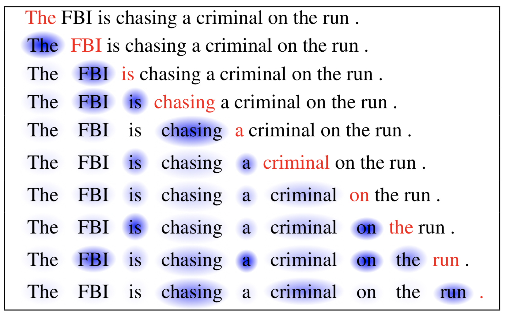
Self-attention, also called intra-attention, is an attention mechanism that relates different positions within a single sequence in order to compute a representation of that same sequence. It has been shown to be valuable for tasks such as machine reading, abstractive summarization, and image description generation.
The long short-term memory network paper applied self-attention to machine reading. In the example below, self-attention makes it possible to learn correlations between the current word and earlier parts of the sentence.
Soft vs Hard Attention
In the show, attend and tell paper, attention is applied to images to generate captions. The image is first encoded by a CNN to extract features. A LSTM decoder then consumes the convolutional features to generate descriptive words sequentially, with weights learned through attention. Visualizing these attention weights makes it clear which image regions the model focuses on when producing a given word.
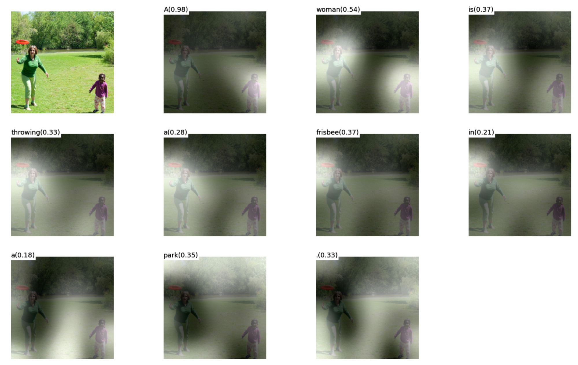
This paper first introduced the “soft” versus “hard” attention distinction, based on whether attention can access the entire image or only a single patch:
- Soft Attention: alignment weights are learned and distributed “softly” across all patches in the source image, essentially the same form as in Bahdanau et al., 2015.
- Pro: the model is smooth and differentiable.
- Con: computationally expensive when the source input is large.
- Hard Attention: selects only one image patch to attend to at a time.
- Pro: less computation during inference.
- Con: non-differentiable, requiring more complex training techniques such as variance reduction or reinforcement learning. (Luong, et al., 2015)
Global vs Local Attention
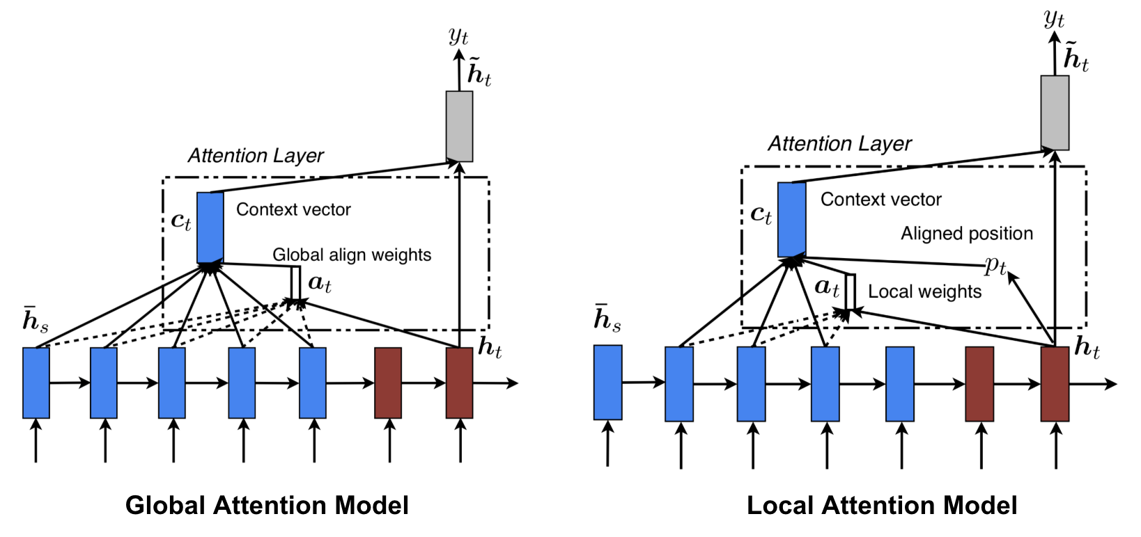
Luong, et al., 2015 proposed the terms “global” and “local” attention. Global attention is similar to soft attention. Local attention, by contrast, is an interesting hybrid of hard and soft, designed as a differentiable improvement over hard attention. The model first predicts a single aligned position for the current target word, then computes a context vector using a window centered around that source position.
Neural Turing Machines
In 1936, Alan Turing proposed a minimalist model of computation. It consists of an infinitely long tape and a head that interacts with the tape. The tape contains countless cells, each holding a symbol: 0, 1, or blank (" “). The head can read symbols, write symbols, and move left or right along the tape. In theory, a Turing machine can simulate any computer algorithm, regardless of how complex or costly the procedure may be. The infinite memory makes the Turing machine mathematically unbounded. However, infinite memory is not feasible in modern physical computers, so the Turing machine is generally treated as a mathematical model of computation.
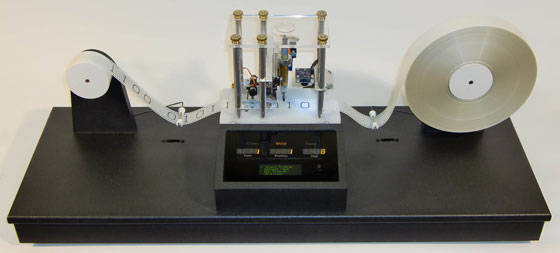
Neural Turing Machine (NTM, Graves, Wayne & Danihelka, 2014) is an architecture that couples a neural network with an external memory store. The memory plays a role similar to the Turing machine tape, and the neural network controls operation heads that read from and write to the tape. In NTM, however, the memory is finite, so it arguably resembles a “Neural von Neumann Machine” more closely.
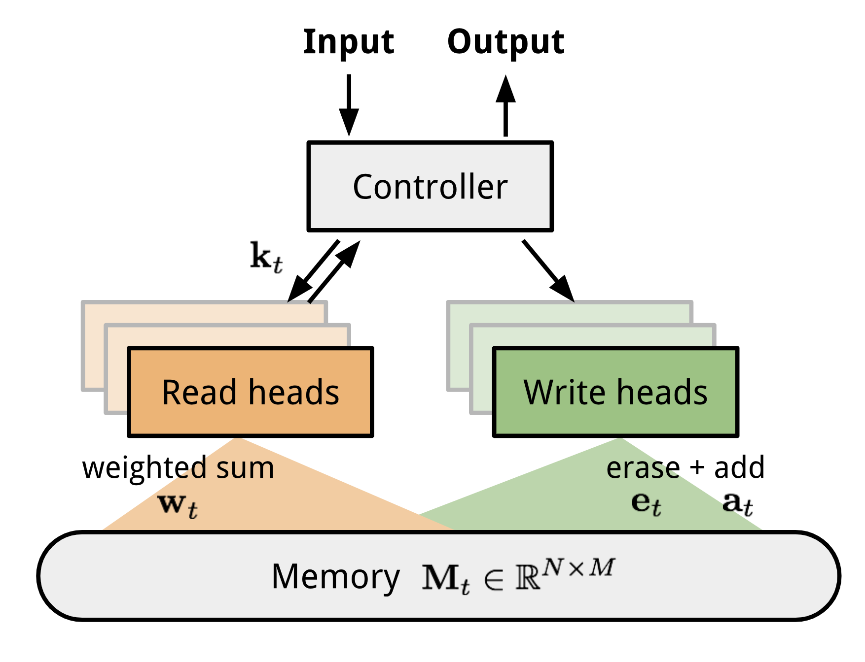
NTM has two primary components: a controller neural network and a memory bank.
Controller: responsible for executing operations on the memory. It may be any neural network type, feed-forward or recurrent.
Memory: stores processed information as a matrix of size $N \times M$, containing N row vectors, each with $M$ dimensions.
During a single update iteration, the controller processes the input and interacts with the memory bank to produce output. This interaction is mediated by a set of parallel read and write heads. Both reading and writing are performed “blurrily”, by softly attending to all memory addresses.
Reading and Writing
When reading from memory at time t, an attention vector of size $N$, $\mathbf{w}_t$ determines how much attention to allocate to each memory location (that is, each matrix row). The read vector $\mathbf{r}_t$ is computed as a weighted sum using the attention intensities:
where $w_t(i)$ is the $i$-th element in $\mathbf{w}_t$ and $\mathbf{M}_t(i)$ is the $i$-th row vector in the memory.
When writing to memory at time t, inspired by the input and forget gates in LSTM, a write head first removes some existing content based on an erase vector $\mathbf{e}_t$, and then incorporates new information using an add vector $\mathbf{a}_t$.
Attention Mechanisms
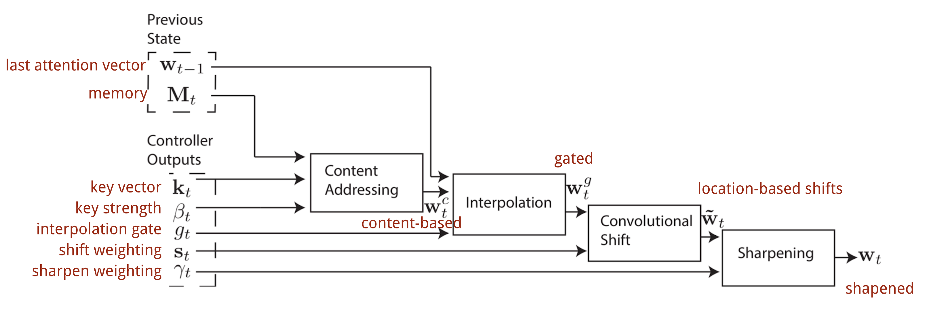
In a Neural Turing Machine, the procedure for producing the attention distribution $\mathbf{w}_t$ depends on the addressing mechanisms. NTM uses a mixture of content-based and location-based addressing.
Content-based addressing
Content-based addressing constructs attention vectors from the similarity between a key vector $\mathbf{k}_t$ (extracted by the controller from the input) and the memory rows. The content-based attention scores are computed via cosine similarity and then normalized with softmax. In addition, NTM includes a strength multiplier $\beta_t$ to sharpen or soften the distribution’s focus.
Interpolation
An interpolation gate scalar $g_t$ then blends the newly computed content-based attention vector with the attention weights from the previous time step:
Location-based addressing
Location-based addressing aggregates values across positions in the attention vector, weighted by a weighting distribution over allowed integer shifts. This is equivalent to a 1-d convolution with a kernel $\mathbf{s}_t(.)$, expressed as a function of the position offset. There are multiple ways to define this distribution. See for inspiration.
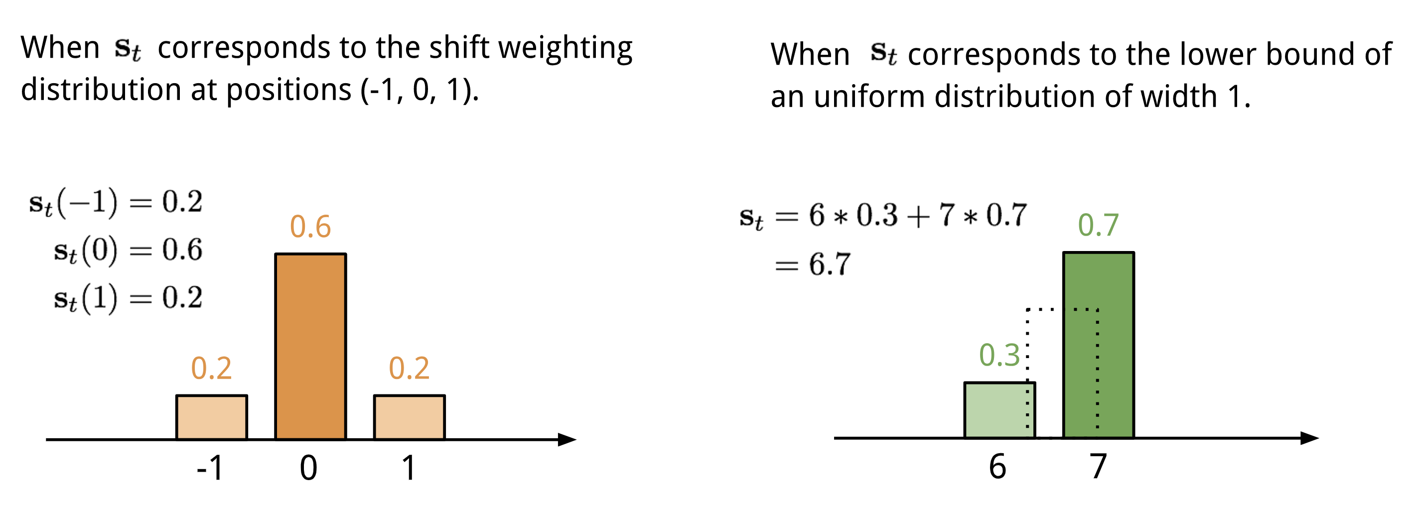
Finally, the attention distribution is sharpened using a scalar $\gamma_t \geq 1$.
The full process for generating the attention vector $\mathbf{w}_t$ at time step t is illustrated in All parameters produced by the controller are unique per head. When multiple read and write heads operate in parallel, the controller outputs multiple parameter sets.
Pointer Network
For problems such as sorting or the travelling salesman problem, both the inputs and outputs are sequential. Unfortunately, classic seq-2-seq or NMT models do not handle these tasks easily, because the discrete categories of output elements are not fixed in advance, but instead depend on the variable input size. The Pointer Net (Ptr-Net; Vinyals, et al. 2015) was proposed to address this setting, where output elements correspond to positions in an input sequence. Instead of using attention to combine encoder hidden units into a context vector (see Fig. 8), Pointer Net applies attention over input elements to select one element as the output at each decoder step.
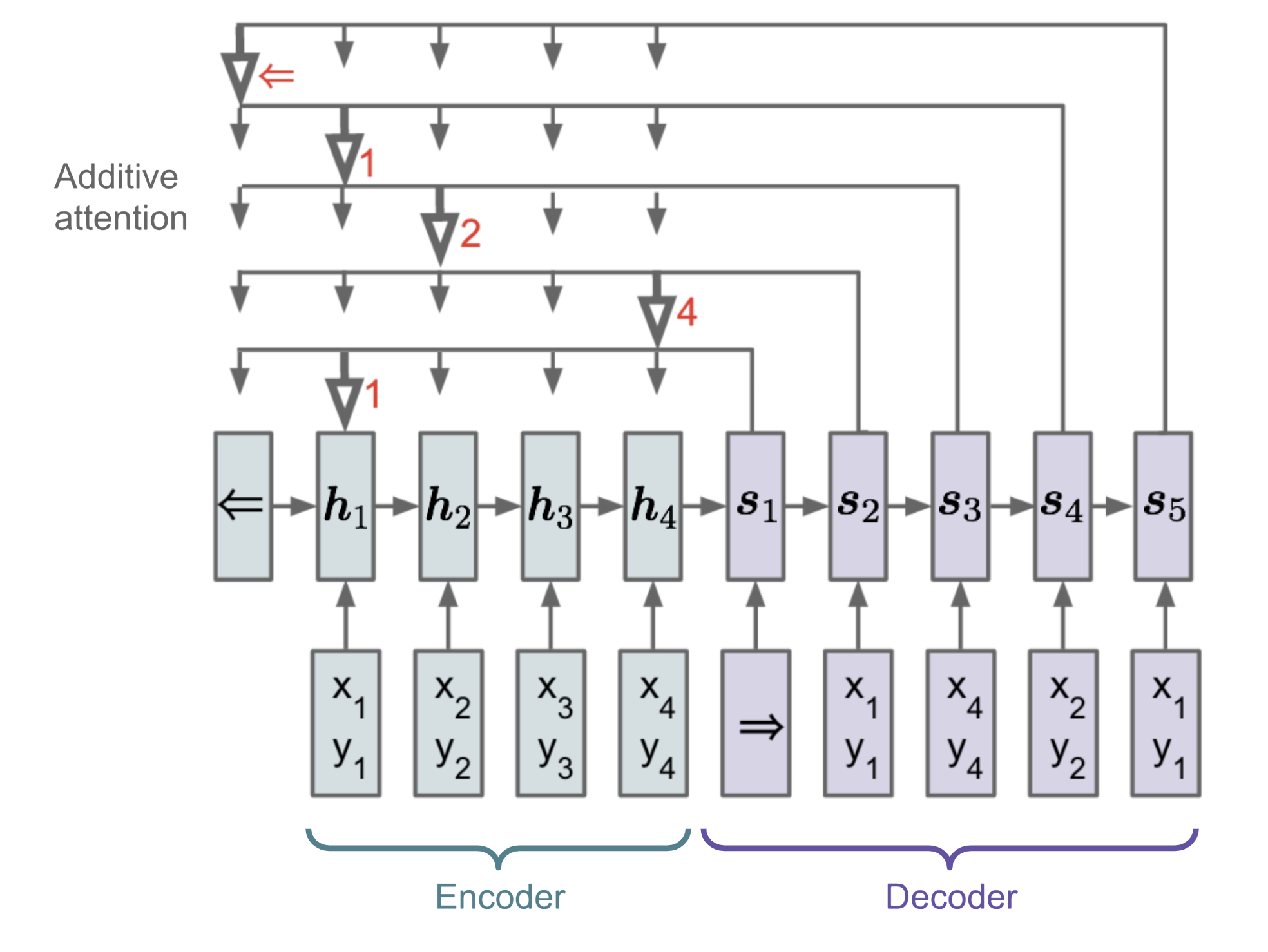
Ptr-Net produces a sequence of integer indices, $\boldsymbol{c} = (c_1, \dots, c_m)$, given a sequence of input vectors $\boldsymbol{x} = (x_1, \dots, x_n)$ and $1 \leq c_i \leq n$. The model still follows an encoder-decoder framework. The encoder and decoder hidden states are $(\boldsymbol{h}_1, \dots, \boldsymbol{h}_n)$ and $(\boldsymbol{s}_1, \dots, \boldsymbol{s}_m)$, respectively. Note that $\mathbf{s}_i$ is the output gate after cell activation in the decoder. Ptr-Net uses additive attention between states and then applies softmax normalization to model the output conditional probability:
This attention mechanism is streamlined because Ptr-Net does not combine encoder states into the output via attention weights. As a result, the output responds only to positions, rather than to the input content.
Transformer
“Attention is All you Need” (Vaswani, et al., 2017) is, without question, one of the most influential and compelling papers of 2017. It introduced multiple improvements to soft attention and demonstrated that sequence-to-sequence modeling can be performed without recurrent units. The proposed transformer model is constructed entirely around self-attention mechanisms, avoiding any sequence-aligned recurrent architecture.
The core insight lies in the model architecture itself.
Key, Value and Query
The transformer’s central building block is the multi-head self-attention mechanism. The model treats an input’s encoded representation as a collection of key-value pairs, $(\mathbf{K}, \mathbf{V})$, each of dimension $n$ (input sequence length). In the neural machine translation setting, both the keys and values correspond to the encoder hidden states. On the decoder side, the previous output is summarized into a query ($\mathbf{Q}$ of dimension $m$), and the next output is generated by mapping this query against the set of keys and values.
The transformer uses scaled dot-product attention. The output is computed as a weighted sum of the values, where each value’s weight is determined by the dot product between the query and every key:
Multi-Head Self-Attention
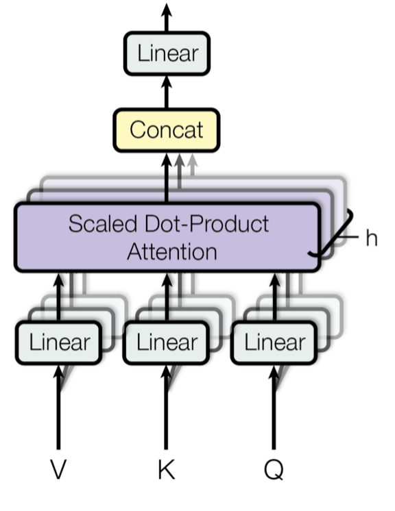
Instead of computing attention a single time, the multi-head approach executes scaled dot-product attention multiple times in parallel. The resulting attention outputs are concatenated and then passed through a linear transformation to obtain the required dimensions. I assume the motivation is because ensembling always helps? ;) As stated in the paper, “multi-head attention allows the model to jointly attend to information from different representation subspaces at different positions. With a single attention head, averaging inhibits this.”
where $\mathbf{W}^Q_i$, $\mathbf{W}^K_i$, $\mathbf{W}^V_i$, and $\mathbf{W}^O$ are learned parameter matrices.
Encoder
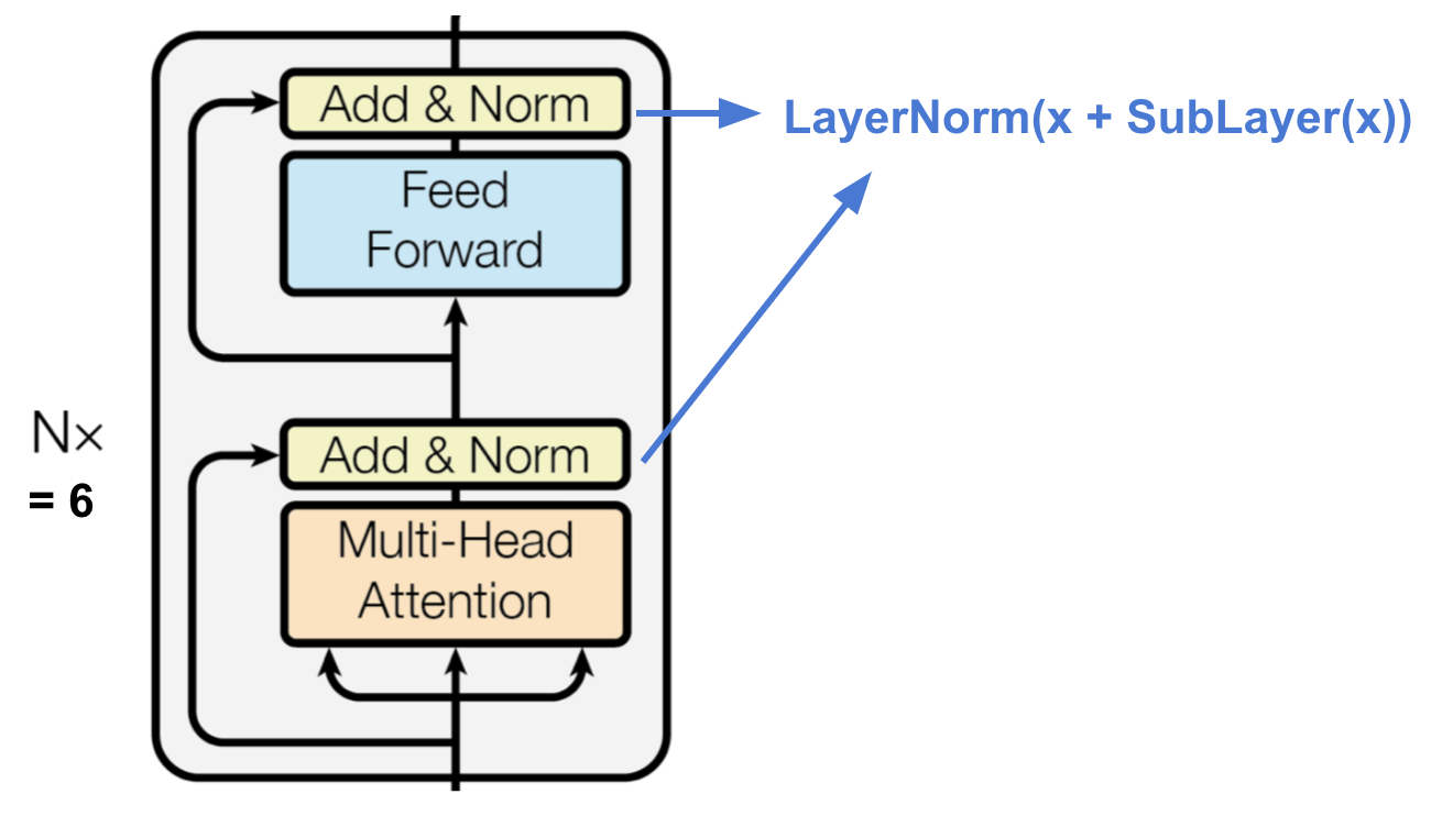
The encoder produces an attention-based representation that can retrieve a specific piece of information from a potentially infinitely large context.
- A stack of N=6 identical layers.
- Each layer contains a multi-head self-attention layer and a position-wise fully connected feed-forward network.
- Each sub-layer uses a residual connection and layer normalization. All sub-layers produce outputs with the same dimensionality, $d_\text{model} = 512$.
Decoder
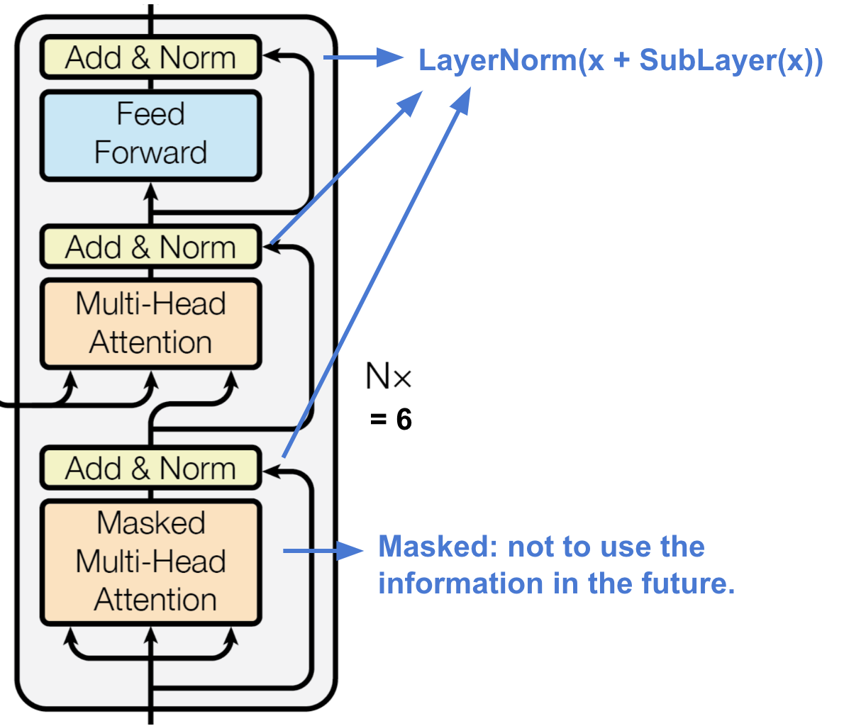
The decoder can retrieve information from the encoded representation.
- A stack of N = 6 identical layers
- Each layer contains two multi-head attention sub-layers and one fully connected feed-forward sub-layer.
- As in the encoder, every sub-layer applies a residual connection and layer normalization.
- The first multi-head attention sub-layer is modified to prevent positions from attending to subsequent positions, since the model must not look ahead in the target sequence when predicting the current position.
Full Architecture
The following summarizes the complete transformer architecture:
- Both source and target sequences are first passed through embedding layers, producing representations with the same dimensionality, $d_\text{model} =512$.
- To retain position information, a sinusoid-wave-based positional encoding is computed and added to the embedding outputs.
- A linear layer and softmax are applied to the final decoder output.
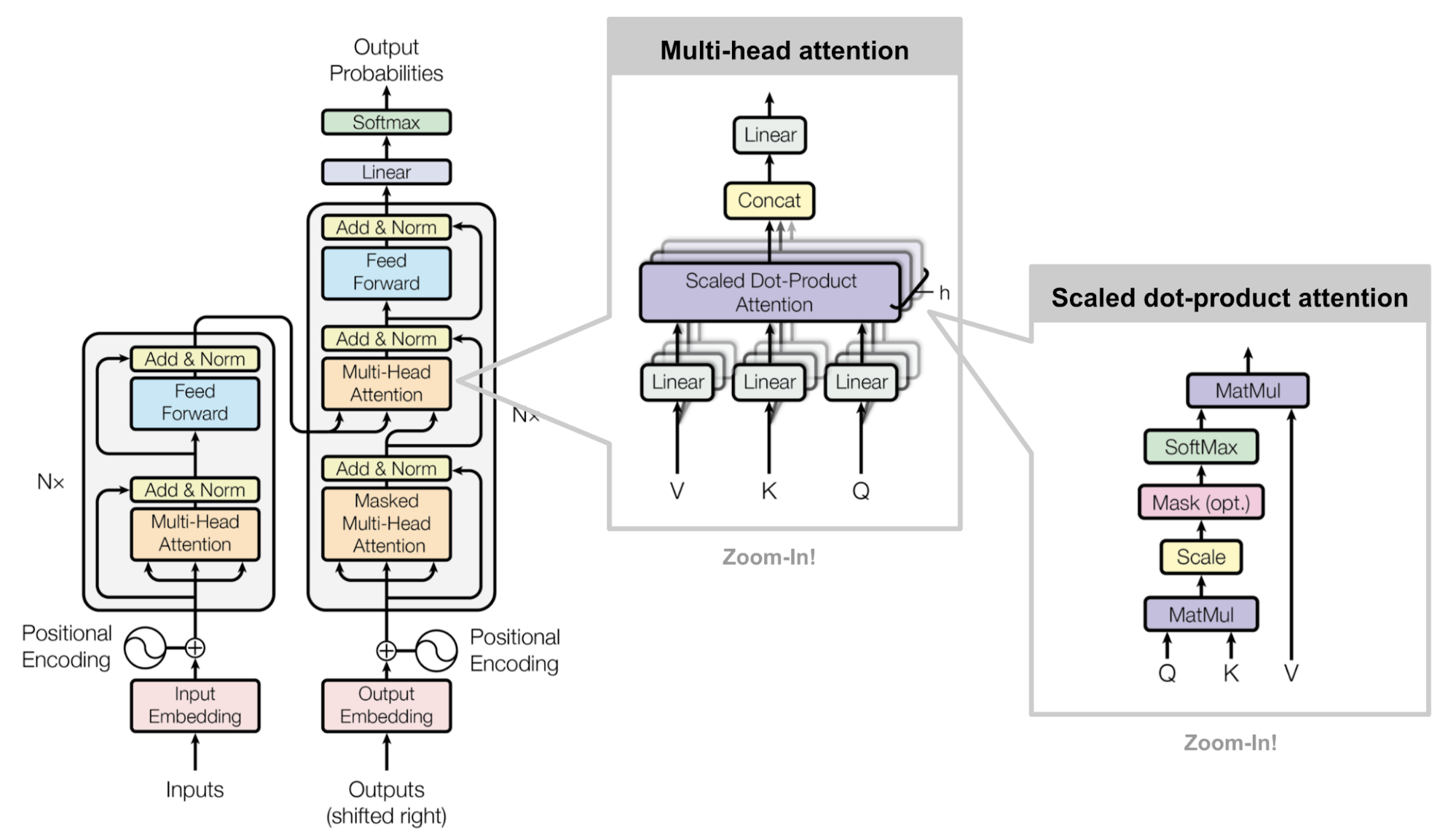
Implementing the transformer model is an interesting experience. Here is my implementation: lilianweng/transformer-tensorflow. If you are interested, see the comments within the code.
SNAIL
The transformer contains neither recurrent nor convolutional structure. Even with positional encoding added to embeddings, sequential order is only weakly represented. For tasks that are sensitive to positional dependencies, such as reinforcement learning, this can present a significant limitation.
The Simple Neural Attention Meta-Learner (SNAIL) (Mishra et al., 2017) was developed in part to address the transformer’s positioning issue by combining the transformer-style self-attention mechanism with temporal convolutions. It has been shown to perform well on both supervised learning and reinforcement learning tasks.
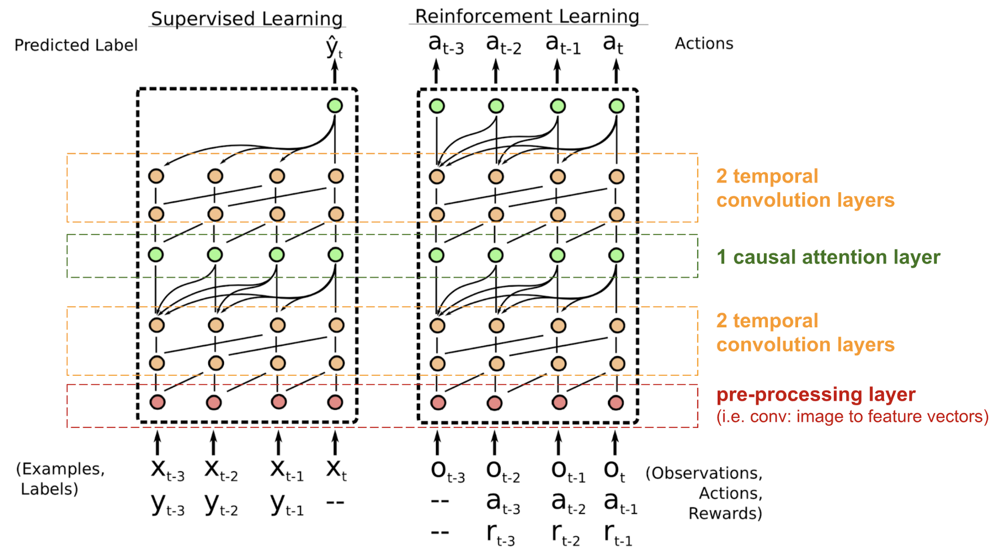
SNAIL originated in meta-learning, a substantial topic that warrants its own post. Put simply, a meta-learning model is expected to generalize to new, unseen tasks drawn from a similar distribution. If you would like more background, see this helpful introduction here.
Self-Attention GAN
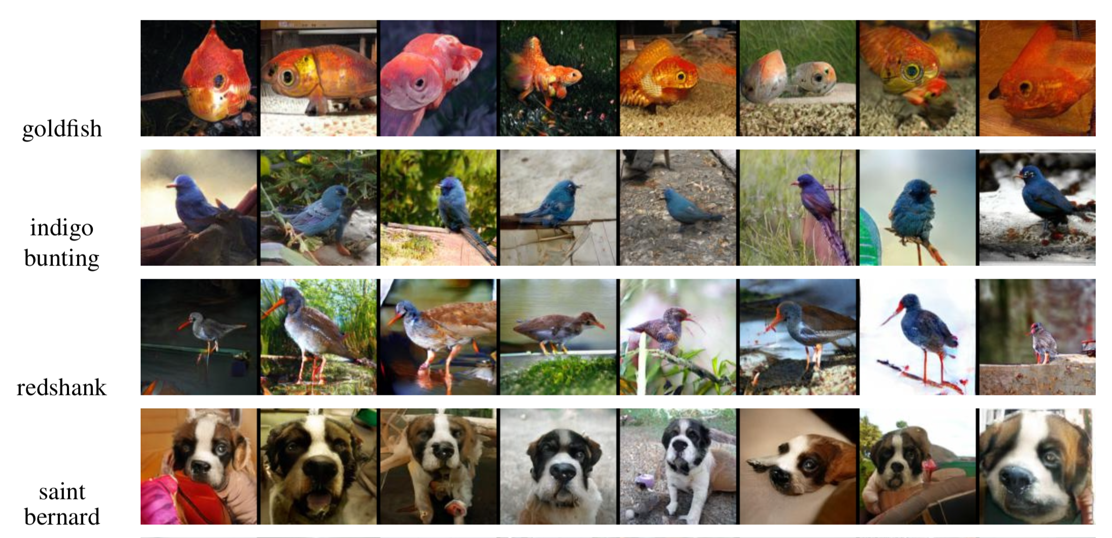
Self-Attention GAN (SAGAN; Zhang et al., 2018) incorporates self-attention layers into GAN so that both the generator and discriminator can model relationships between spatial regions more effectively.
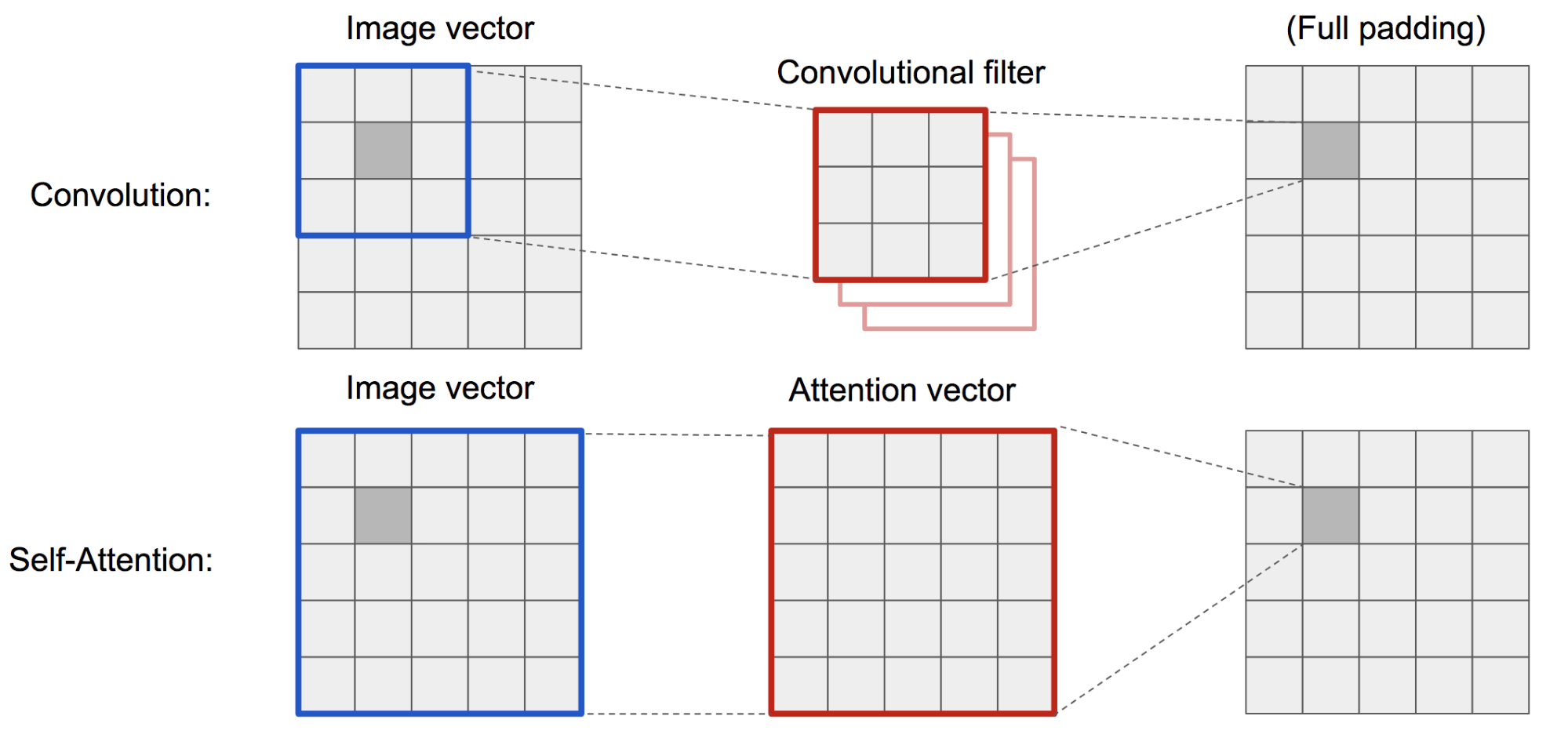
The classic DCGAN (Deep Convolutional GAN) implements both the discriminator and generator as multi-layer convolutional networks. However, representational capacity is constrained by filter size, because each pixel’s feature is limited to a small local neighborhood. To relate distant regions, features must be propagated through multiple convolution layers, and the resulting dependencies are not guaranteed to be preserved.
Because (soft) self-attention in vision is explicitly designed to learn relationships between one pixel and all other locations, including distant regions, it can capture global dependencies more directly. Therefore, a GAN equipped with self-attention is expected to handle details better, hooray!
SAGAN adopts the non-local neural network formulation for attention computation. The convolutional image feature maps $\mathbf{x}$ are branched into three copies, corresponding to key, value, and query in the transformer:
- Key: $f(\mathbf{x}) = \mathbf{W}_f \mathbf{x}$
- Query: $g(\mathbf{x}) = \mathbf{W}_g \mathbf{x}$
- Value: $h(\mathbf{x}) = \mathbf{W}_h \mathbf{x}$
Dot-product attention is then applied to produce the self-attention feature maps:
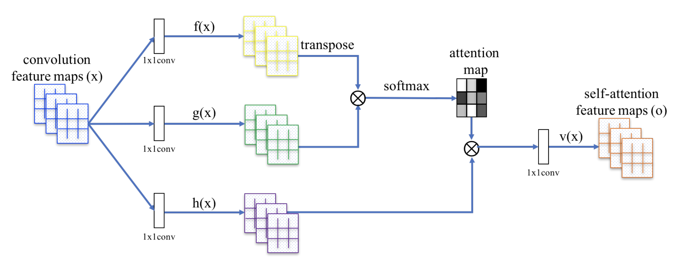
Note that $\alpha_{i,j}$ is a single entry in the attention map. It represents how much attention the model should assign to the $i$-th position when synthesizing the $j$-th location. $\mathbf{W}_f$, $\mathbf{W}_g$, and $\mathbf{W}_h$ are 1x1 convolution filters. If 1x1 conv feels like a strange concept (for example, is it not simply multiplying the entire feature map by a single number?), see this short tutorial by Andrew Ng. The output $\mathbf{o}_j$ is a column vector representing the final output $\mathbf{o}= (\mathbf{o}_1, \mathbf{o}_2, \dots, \mathbf{o}_j, \dots, \mathbf{o}_N)$.
In addition, the attention layer output is multiplied by a scale parameter and added back to the original input feature map:
During training, the scaling parameter $\gamma$ is gradually increased from 0. This encourages the network to rely first on local cues and then progressively learn to place more weight on regions that are farther away.
Cited as:
@article{weng2018attention,
  title   = "Attention? Attention!",
  author  = "Weng, Lilian",
  journal = "lilianweng.github.io",
  year    = "2018",
  url     = "https://lilianweng.github.io/posts/2018-06-24-attention/"
}
References
[1] “Attention and Memory in Deep Learning and NLP.” - Jan 3, 2016 by Denny Britz
[2] “Neural Machine Translation (seq2seq) Tutorial”
[3] Dzmitry Bahdanau, Kyunghyun Cho, and Yoshua Bengio. “Neural machine translation by jointly learning to align and translate.” ICLR 2015.
[4] Kelvin Xu, Jimmy Ba, Ryan Kiros, Kyunghyun Cho, Aaron Courville, Ruslan Salakhudinov, Rich Zemel, and Yoshua Bengio. “Show, attend and tell: Neural image caption generation with visual attention.” ICML, 2015.
[5] Ilya Sutskever, Oriol Vinyals, and Quoc V. Le. “Sequence to sequence learning with neural networks.” NIPS 2014.
[6] Thang Luong, Hieu Pham, Christopher D. Manning. “Effective Approaches to Attention-based Neural Machine Translation.” EMNLP 2015.
[7] Denny Britz, Anna Goldie, Thang Luong, and Quoc Le. “Massive exploration of neural machine translation architectures.” ACL 2017.
[8] Ashish Vaswani, et al. “Attention is all you need.” NIPS 2017.
[9] Jianpeng Cheng, Li Dong, and Mirella Lapata. “Long short-term memory-networks for machine reading.” EMNLP 2016.
[10] Xiaolong Wang, et al. “Non-local Neural Networks.” CVPR 2018
[11] Han Zhang, Ian Goodfellow, Dimitris Metaxas, and Augustus Odena. “Self-Attention Generative Adversarial Networks.” arXiv preprint arXiv:1805.08318 (2018).
[12] Nikhil Mishra, Mostafa Rohaninejad, Xi Chen, and Pieter Abbeel. “A simple neural attentive meta-learner.” ICLR 2018.
[13] “WaveNet: A Generative Model for Raw Audio” - Sep 8, 2016 by DeepMind.
[14] Oriol Vinyals, Meire Fortunato, and Navdeep Jaitly. “Pointer networks.” NIPS 2015.
[15] Alex Graves, Greg Wayne, and Ivo Danihelka. “Neural turing machines.” arXiv preprint arXiv:1410.5401 (2014).