The objective of contrastive representation learning is to construct an embedding space where similar sample pairs remain nearby and dissimilar pairs are pushed far apart. Contrastive learning can be used in both supervised and unsupervised settings. In the unsupervised case, it is among the most effective techniques in self-supervised learning.

Contrastive Training Objectives

Early contrastive-learning loss functions typically used only a single positive and a single negative sample. More recent objectives increasingly incorporate multiple positive and negative pairs within a single batch.

Contrastive Loss

Contrastive loss (Chopra et al. 2005) is one of the earliest objectives used for deep metric learning via a contrastive formulation.

Given a collection of input samples $\{ \mathbf{x}_i \}$, each sample has an associated label $y_i \in \{1, \dots, L\}$ drawn from $L$ classes. We aim to learn a function $f_\theta(.): \mathcal{X}\to\mathbb{R}^d$ that maps $x_i$ to an embedding vector, such that samples from the same class produce similar embeddings, while samples from different classes produce substantially different embeddings. Accordingly, contrastive loss considers a pair of inputs $(x_i, x_j)$, minimizing the embedding distance when the two inputs share a class label and maximizing it otherwise.

where $\epsilon$ is a hyperparameter that specifies the minimum (lower-bound) distance between samples from different classes.

Triplet Loss

Triplet loss was introduced in the FaceNet paper (Schroff et al. 2015) and was applied to learning face recognition for the same person across varying poses and angles.

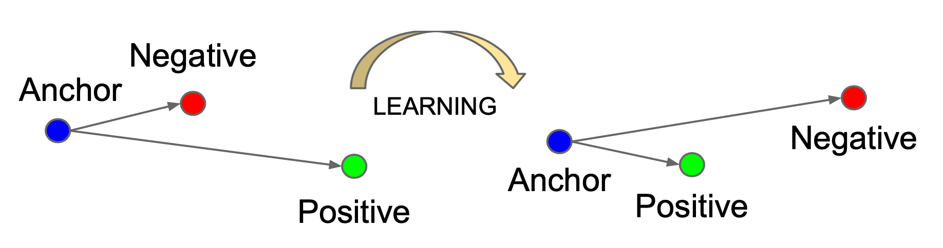
Given an anchor input $\mathbf{x}$, we choose one positive sample $\mathbf{x}^+$ and one negative $\mathbf{x}^-$. Here, $\mathbf{x}^+$ and $\mathbf{x}$ come from the same class, while $\mathbf{x}^-$ is sampled from a different class. Triplet loss simultaneously learns to reduce the distance between the anchor $\mathbf{x}$ and the positive $\mathbf{x}^+$, and to increase the distance between the anchor $\mathbf{x}$ and the negative $\mathbf{x}^-$, using the following formulation:

where the margin parameter $\epsilon$ sets the minimum required separation between distances for similar versus dissimilar pairs.

Selecting challenging $\mathbf{x}^-$ is essential for meaningfully improving the model.

Lifted Structured Loss

Lifted Structured Loss (Song et al. 2015) leverages all pairwise edges within a training batch to improve computational efficiency.

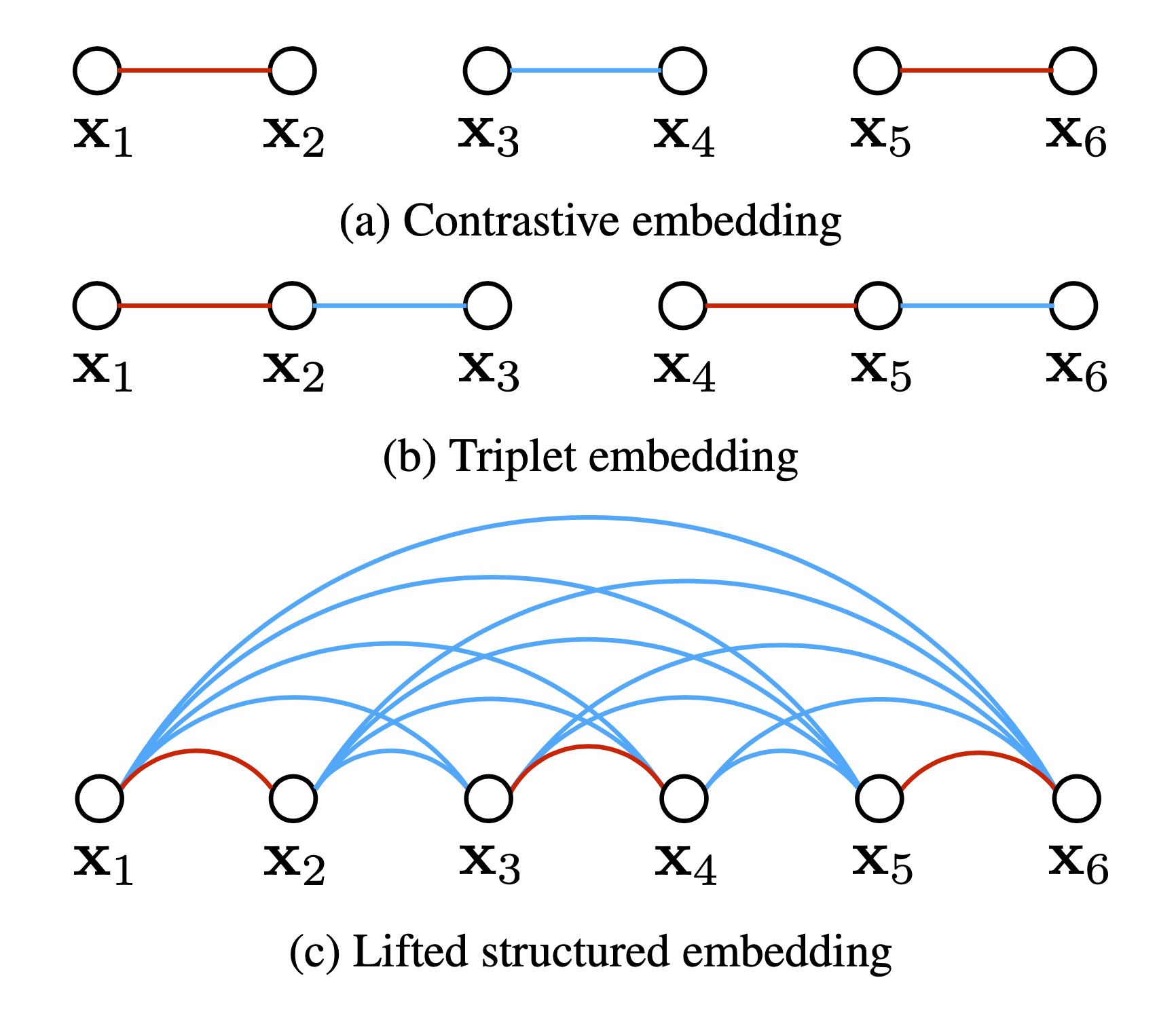
Let $D_{ij} = | f(\mathbf{x}_i) - f(\mathbf{x}_j) |_2$, a structured loss is defined as:

where $\mathcal{P}$ denotes the set of positive pairs and $\mathcal{N}$ denotes the set of negative pairs. Note that the dense pairwise squared-distance matrix can be computed efficiently for each training batch.

The red component in $\mathcal{L}_\text{struct}^{(ij)}$ is used to mine hard negatives. However, because it is not smooth, it may lead in practice to convergence at a poor local optimum. Therefore, it is relaxed as follows:

The paper also proposes improving the quality of negative samples within each batch by actively incorporating difficult negative examples, given a few randomly selected positive pairs.

N-pair Loss

Multi-Class N-pair loss (Sohn 2016) extends triplet loss by comparing against multiple negative samples.

Given a $(N + 1)$-tuplet of training samples, $\{ \mathbf{x}, \mathbf{x}^+, \mathbf{x}^-_1, \dots, \mathbf{x}^-_{N-1} \}$, consisting of one positive and $N-1$ negative samples, the N-pair loss is defined as:

If only one negative is sampled per class, this becomes equivalent to the softmax loss for multi-class classification.

NCE

Noise Contrastive Estimation, abbreviated as NCE, is a technique for estimating the parameters of a statistical model, introduced by Gutmann & Hyvarinen in 2010. The approach trains a logistic regression classifier to distinguish target data from noise. For additional details on the use of NCE in learning word embeddings, see here.

Let $\mathbf{x}$ denote the target sample $\sim P(\mathbf{x} \vert C=1; \theta) = p_\theta(\mathbf{x})$ and $\tilde{\mathbf{x}}$ denote the noise sample $\sim P(\tilde{\mathbf{x}} \vert C=0) = q(\tilde{\mathbf{x}})$. Recall that logistic regression models the logit (that is, the log-odds). In this setting, we model the logit that a sample $u$ originates from the target data distribution rather than the noise distribution:

After converting logits to probabilities using the sigmoid $\sigma(.)$, we apply the cross-entropy loss:

This is the original NCE loss form, which uses only one positive and one noise sample. In many later works, contrastive objectives that incorporate multiple negative samples are also commonly referred to as NCE.

InfoNCE

The InfoNCE loss in CPC (Contrastive Predictive Coding; van den Oord, et al. 2018), inspired by NCE, uses categorical cross-entropy to identify the positive sample among a set of unrelated noise samples.

Given a context vector $\mathbf{c}$, the positive sample is drawn from the conditional distribution $p(\mathbf{x} \vert \mathbf{c})$, while $N-1$ negative samples are drawn from the proposal distribution $p(\mathbf{x})$ and are independent of the context $\mathbf{c}$. For convenience, label all samples as $X=\{ \mathbf{x}_i \}^N_{i=1}$, where exactly one sample $\mathbf{x}_\texttt{pos}$ is positive. The probability of correctly detecting the positive sample is:

where the scoring function is $f(\mathbf{x}, \mathbf{c}) \propto \frac{p(\mathbf{x}\vert\mathbf{c})}{p(\mathbf{x})}$.

InfoNCE optimizes the negative log probability of correctly classifying the positive sample:

The observation that $f(x, c)$ estimates the density ratio $\frac{p(x\vert c)}{p(x)}$ connects this objective to mutual-information optimization. To maximize the mutual information between input $x$ and context vector $c$, we have:

where the logarithmic term shown in blue is estimated by $f$.

For sequence prediction tasks, instead of directly modeling future observations $p_k(\mathbf{x}_{t+k} \vert \mathbf{c}_t)$ (which can be computationally expensive), CPC models a density function to preserve the mutual information between $\mathbf{x}_{t+k}$ and $\mathbf{c}_t$:

where $\mathbf{z}_{t+k}$ is the encoded input and $\mathbf{W}_k$ is a trainable weight matrix.

Soft-Nearest Neighbors Loss

Soft-Nearest Neighbors Loss (Salakhutdinov & Hinton 2007, Frosst et al. 2019) extends the approach to incorporate multiple positive samples.

Given a batch of samples, $\{\mathbf{x}_i, y_i)\}^B_{i=1}$, where $y_i$ is the class label of $\mathbf{x}_i$, and a similarity function $f(.,.)$ between two inputs, the soft nearest neighbor loss at temperature $\tau$ is:

The temperature $\tau$ controls how concentrated features become in the representation space. For instance, at low temperature the loss is dominated by small distances, and widely separated representations contribute little and can effectively become irrelevant.

Common Setup

In soft nearest-neighbor loss, the notions of “classes” and “labels” can be broadened to form positive and negative pairs from unsupervised data, for example by using data augmentation to create noisy versions of the original samples.

Many recent works adopt the following contrastive objective setup to support multiple positive and negative samples. Following (Wang & Isola 2020), let $p_\texttt{data}(.)$ be the data distribution over $\mathbb{R}^n$, and let $p_\texttt{pos}(., .)$ be the distribution of positive pairs over $\mathbb{R}^{n \times n}$. These distributions must satisfy:

• Symmetry: $\forall \mathbf{x}, \mathbf{x}^+, p_\texttt{pos}(\mathbf{x}, \mathbf{x}^+) = p_\texttt{pos}(\mathbf{x}^+, \mathbf{x})$
• Matching marginal: $\forall \mathbf{x}, \int p_\texttt{pos}(\mathbf{x}, \mathbf{x}^+) d\mathbf{x}^+ = p_\texttt{data}(\mathbf{x})$

To learn an encoder $f(\mathbf{x})$ that produces an L2-normalized feature vector, the contrastive learning objective is:

Key Ingredients

Heavy Data Augmentation

For each training sample, data augmentation is used to generate noisy variants that can be treated as positive samples in the loss. A well-designed augmentation pipeline is critical to learning embedding features that are both strong and generalizable. Augmentations introduce non-essential variation without changing semantic meaning, encouraging the model to capture what is essential in the representation. For example, SimCLR experiments showed that combining random cropping with random color distortion is crucial for high performance in learning visual image representations.

Large Batch Size

Training with a large batch size is another key factor behind the success of many contrastive methods (for example, SimCLR and CLIP), particularly when using in-batch negatives. Only with sufficiently large batches can the loss span a diverse and challenging set of negative samples, enabling the model to learn representations that reliably distinguish between different examples.

Hard Negative Mining

Hard negatives are samples with labels different from the anchor, yet whose embedding features lie very close to the anchor embedding. With ground-truth labels available in supervised datasets, identifying task-specific hard negatives is straightforward. For example, in sentence embedding learning, sentence pairs labeled as “contradiction” in NLI datasets can be used as hard negatives (for example, SimCSE), or one can use top incorrect candidates returned by BM25 that match most keywords as hard negatives (DPR; Karpukhin et al., 2020).

Hard negative mining becomes more challenging in fully unsupervised settings. Increasing the training batch size or the memory bank size implicitly introduces more hard negatives, but it also imposes substantial memory overhead.

Chuang et al. (2020) analyzed sampling bias in contrastive learning and proposed a debiased loss. In unsupervised settings, because ground-truth labels are unavailable, false negatives may be sampled inadvertently, and this sampling bias can cause a substantial drop in performance.

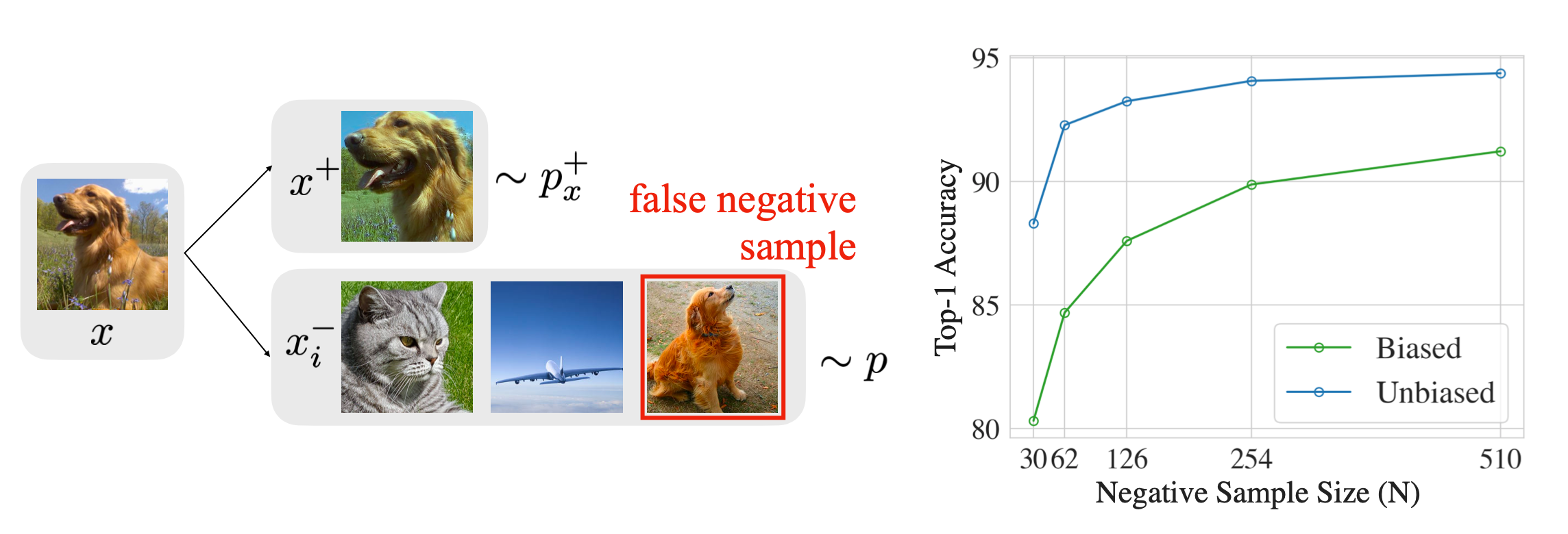
Assume the anchor class probability $c$ is uniform $\rho(c)=\eta^+$, and the probability of observing a different class is $\eta^- = 1-\eta^+$.

• The probability of observing a positive example for $\mathbf{x}$ is $p^+_x(\mathbf{x}’)=p(\mathbf{x}’\vert \mathbf{h}_{x’}=\mathbf{h}_x)$;
• The probability of obtaining a negative sample for $\mathbf{x}$ is $p^-_x(\mathbf{x}’)=p(\mathbf{x}’\vert \mathbf{h}_{x’}\neq\mathbf{h}_x)$.

When sampling $\mathbf{x}^-$, we cannot access the true $p^-_x(\mathbf{x}^-)$. As a result, $\mathbf{x}^-$ may be drawn from the (undesired) anchor class $c$ with probability $\eta^+$. The effective sampling distribution becomes:

Therefore, we can use $p^-_x(\mathbf{x}’) = (p(\mathbf{x}’) - \eta^+ p^+_x(\mathbf{x}’))/\eta^-$ for sampling $\mathbf{x}^-$ to debias the loss. With $N$ samples $\{\mathbf{u}_i\}^N_{i=1}$ from $p$ and $M$ samples $\{ \mathbf{v}_i \}_{i=1}^M$ from $p^+_x$, we can estimate the expectation of the second term $\mathbb{E}_{\mathbf{x}^-\sim p^-_x}[\exp(f(\mathbf{x})^\top f(\mathbf{x}^-))]$ in the denominator of the contrastive learning loss:

where $\tau$ is the temperature and $\exp(-1/\tau)$ is the theoretical lower bound of $\mathbb{E}_{\mathbf{x}^-\sim p^-_x}[\exp(f(\mathbf{x})^\top f(\mathbf{x}^-))]$.

The resulting debiased contrastive loss is:

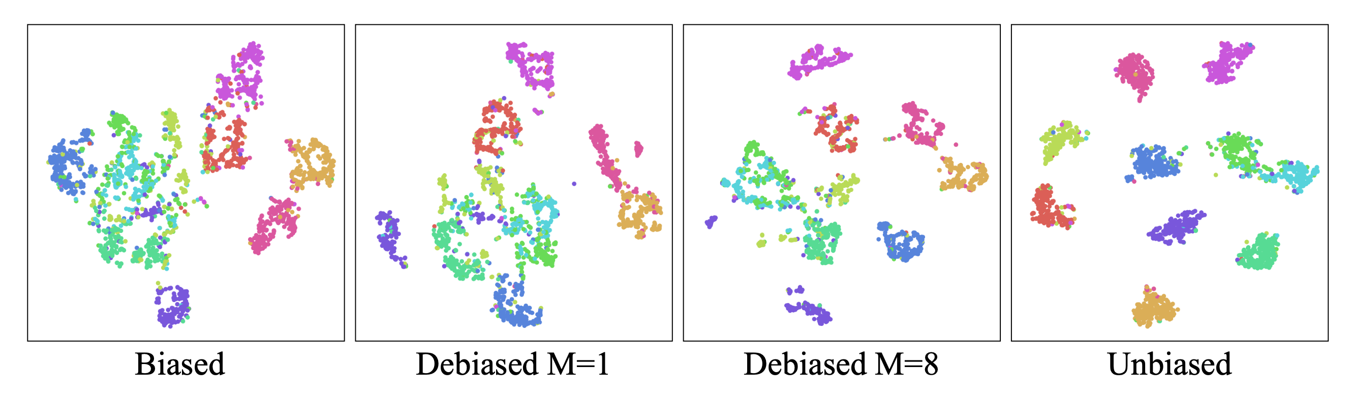
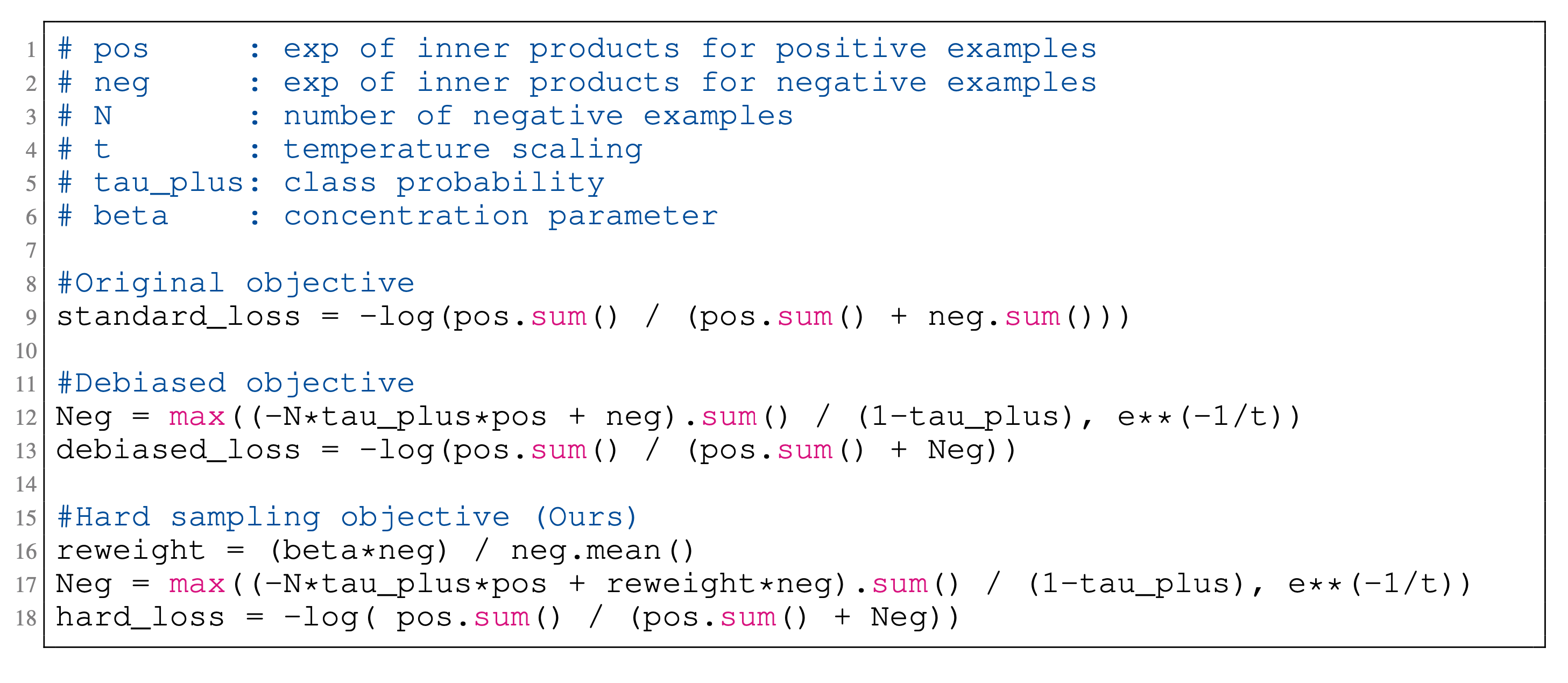
Building on the above notation, Robinson et al. (2021) adjusted the sampling probabilities to focus on hard negatives by increasing the probability $p^-_x(x’)$ in proportion to its similarity to the anchor. The revised sampling probability $q_\beta(x^-)$ is:

where $\beta$ is a tunable hyperparameter.

We can estimate the second denominator term $\mathbb{E}_{\mathbf{x}^- \sim q_\beta} [\exp(f(\mathbf{x})^\top f(\mathbf{x}^-))]$ using importance sampling, where both partition functions $Z_\beta, Z^+_\beta$ can be estimated empirically.

Vision: Image Embedding

Image Augmentations

Most contrastive representation learning methods in vision rely on generating a noisy variant of each sample by applying a sequence of augmentations. The augmentations should substantially change the image’s appearance while preserving its semantic meaning.

Basic Image Augmentation

Many image transformations preserve semantic meaning. Any of the following augmentations, or compositions of multiple operations, can be used:

• Random cropping, followed by resizing back to the original dimensions.
• Random color distortions
• Random Gaussian blur
• Random color jittering
• Random horizontal flip
• Random grayscale conversion
• Multi-crop augmentation: Use two standard resolution crops and sample a set of additional low resolution crops that cover only small parts of the image. Using low resolution crops reduces the compute cost. (SwAV)
• And many more …

Augmentation Strategies

A number of frameworks are designed to learn effective data augmentation strategies (that is, compositions of multiple transforms). Common examples include:

• AutoAugment (Cubuk, et al. 2018): Motivated by NAS, AutoAugment formulates the search for effective augmentation operations (for example, shearing, rotation, invert, and others) for image classification as an RL problem, and seeks the combination that yields the highest evaluation accuracy.
• RandAugment (Cubuk et al., 2019): RandAugment significantly reduces AutoAugment’s search space by controlling the magnitudes of different transformation operations with a single magnitude parameter.
• PBA (Population based augmentation; Ho et al., 2019): PBA combines PBT (Jaderberg et al, 2017) with AutoAugment, using an evolutionary algorithm to train a population of child models in parallel and evolve effective augmentation strategies.
• UDA (Unsupervised Data Augmentation; Xie et al., 2019): From a set of candidate augmentation strategies, UDA selects those that minimize the KL divergence between the predicted distribution for an unlabeled example and the predicted distribution for its unlabeled augmented counterpart.

Image Mixture

Image-mixture methods create new training examples by combining existing data points.

• Mixup (Zhang et al., 2018): Mixup performs a global mixture by forming a weighted, pixel-wise combination of two images $I_1$ and $I_2$: $I_\text{mixup} \gets \alpha I_1 + (1-\alpha) I_2$ and $\alpha \in [0, 1]$.
• Cutmix (Yun et al., 2019): Cutmix performs region-level mixing by constructing a new sample that combines a local region from one image with the remainder of another. $I_\text{cutmix} \gets \mathbf{M}_b \odot I_1 + (1-\mathbf{M}_b) \odot I_2$, where $\mathbf{M}_b \in \{0, 1\}^I$ is a binary mask and $\odot$ denotes element-wise multiplication. This is equivalent to filling the cutout (DeVries & Taylor 2017) region with the corresponding region from another image.
• MoCHi (“Mixing of Contrastive Hard Negatives”; Kalantidis et al. 2020): Given a query $\mathbf{q}$, MoCHi maintains a queue of $K$ negative features $Q=\{\mathbf{n}_1, \dots, \mathbf{n}_K \}$ and orders them by similarity to the query, $\mathbf{q}^\top \mathbf{n}$, in descending order. The first $N$ elements in the queue are treated as the hardest negatives, $Q^N$. Synthetic hard examples are then produced via $\mathbf{h} = \tilde{\mathbf{h}} / |\tilde{\mathbf{h}}|$ where $\tilde{\mathbf{h}} = \alpha\mathbf{n}_i + (1-\alpha) \mathbf{n}_j$ and $\alpha \in (0, 1)$. Even harder samples can be generated by mixing with the query feature, $\mathbf{h}’ = \tilde{\mathbf{h}’} / |\tilde{\mathbf{h}’}|_2$ where $\tilde{\mathbf{h}’} = \beta\mathbf{q} + (1-\beta) \mathbf{n}_j$ and $\beta \in (0, 0.5)$.

Parallel Augmentation

Methods in this category generate two noisy (augmented) versions of a single anchor image, then learn representations so that both augmented samples map to the same embedding.

SimCLR

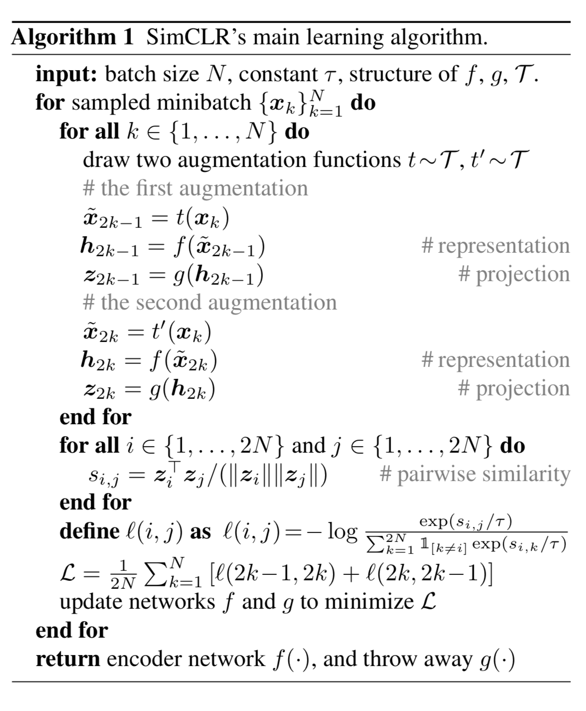
SimCLR (Chen et al, 2020) introduced a straightforward framework for contrastive learning of visual representations. It learns representations for visual inputs by maximizing agreement between differently augmented views of the same sample, using a contrastive loss in latent space.

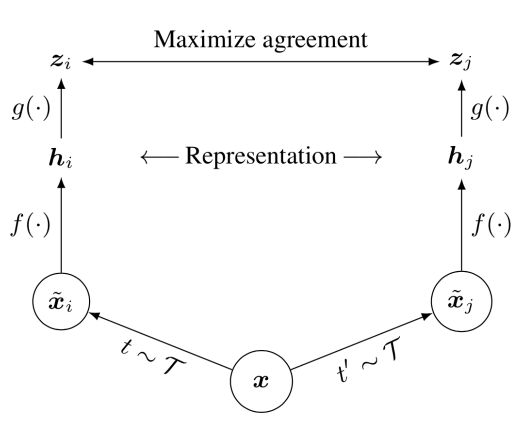
1. Randomly sample a minibatch of $N$ samples. Apply two distinct data augmentation operations to each sample, yielding $2N$ augmented samples in total.

Here, two independent augmentation operators, $t$ and $t’$, are sampled from the same augmentation family $\mathcal{T}$. The data augmentation pipeline includes random crop, resize with random flip, color distortions, and Gaussian blur.

2. For a given positive pair, the remaining $2(N-1)$ data points are treated as negative samples. The representation is produced by a base encoder $f(.)$:

3. The contrastive learning objective is defined using cosine similarity $\text{sim}(.,.)$. Note that the loss is computed on an additional projection layer of the representation, $g(.)$, rather than directly in the representation space. However, only the representation $\mathbf{h}$ is used for downstream tasks.

In this expression, $\mathbb{1}_{[k \neq i]}$ is an indicator function: it equals 1 if $k\neq i$, and 0 otherwise.

SimCLR requires a large batch size so that enough negative samples are available to achieve strong performance.

Barlow Twins

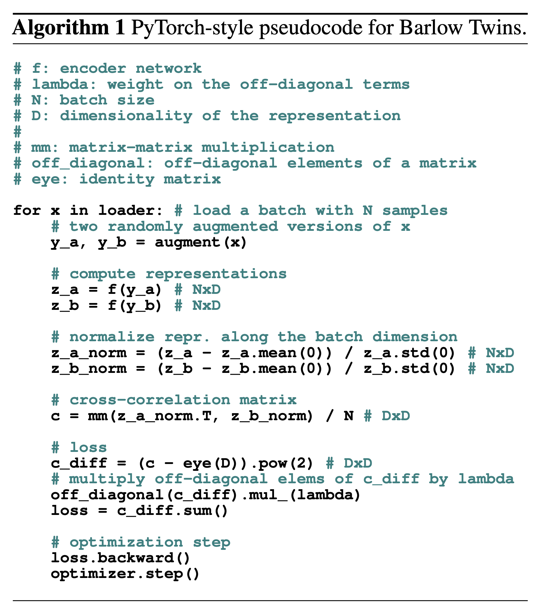
Barlow Twins (Zbontar et al. 2021) feeds two distorted versions of each sample into the same network to extract features, then trains the model so that the cross-correlation matrix between the two sets of output features is close to the identity matrix. The objective is to keep representation vectors from different distortions of the same sample similar, while also reducing redundancy among the representation dimensions.

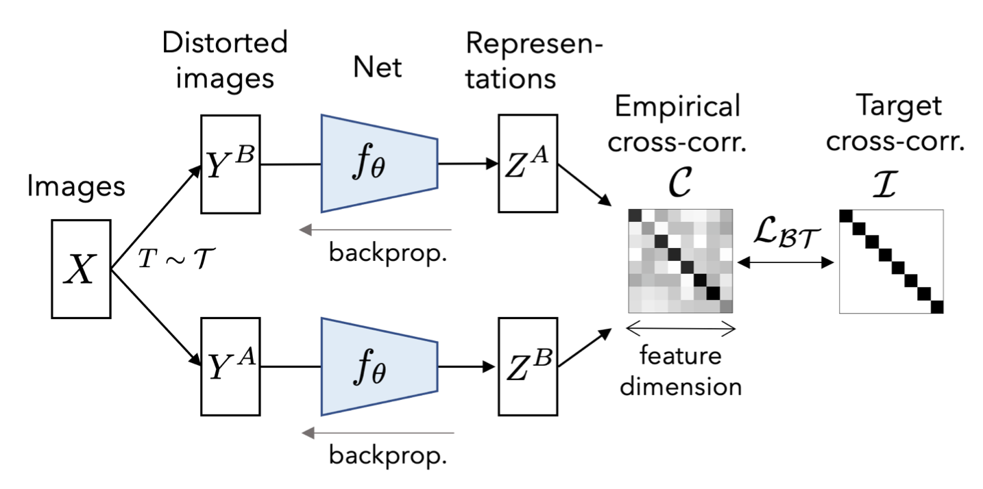
Let $\mathcal{C}$ denote the cross-correlation matrix computed between the outputs of two identical networks along the batch dimension. $\mathcal{C}$ is a square matrix whose size matches the output dimensionality of the feature network. Each entry $\mathcal{C}_{ij}$ is the cosine similarity between the network output dimension indexed by $i, j$ and the batch index $b$, $\mathbf{z}_{b,i}^A$ and $\mathbf{z}_{b,j}^B$, taking values between -1 (perfect anti-correlation) and 1 (perfect correlation).

Barlow Twins is competitive with SOTA self-supervised learning methods. It naturally avoids trivial constant solutions (that is, collapsed representations) and remains robust across different training batch sizes.

BYOL

In contrast to the approaches above, BYOL (Bootstrap Your Own Latent; Grill, et al 2020) claims a new state-of-the-art result without using negative samples. It uses two neural networks, referred to as the online and target networks, which interact and learn from each other. The target network (parameterized by $\xi$) shares the same architecture as the online network (parameterized by $\theta$), but its weights are Polyak-averaged, $\xi \leftarrow \tau \xi + (1-\tau) \theta$.

The objective is to learn a representation $y$ that is useful for downstream tasks. The online network, parameterized by $\theta$, consists of:

• An encoder $f_\theta$;
• A projector $g_\theta$;
• A predictor $q_\theta$.

The target network uses the same architecture, but with a different parameter set $\xi$, updated via Polyak averaging $\theta$: $\xi \leftarrow \tau \xi + (1-\tau) \theta$.

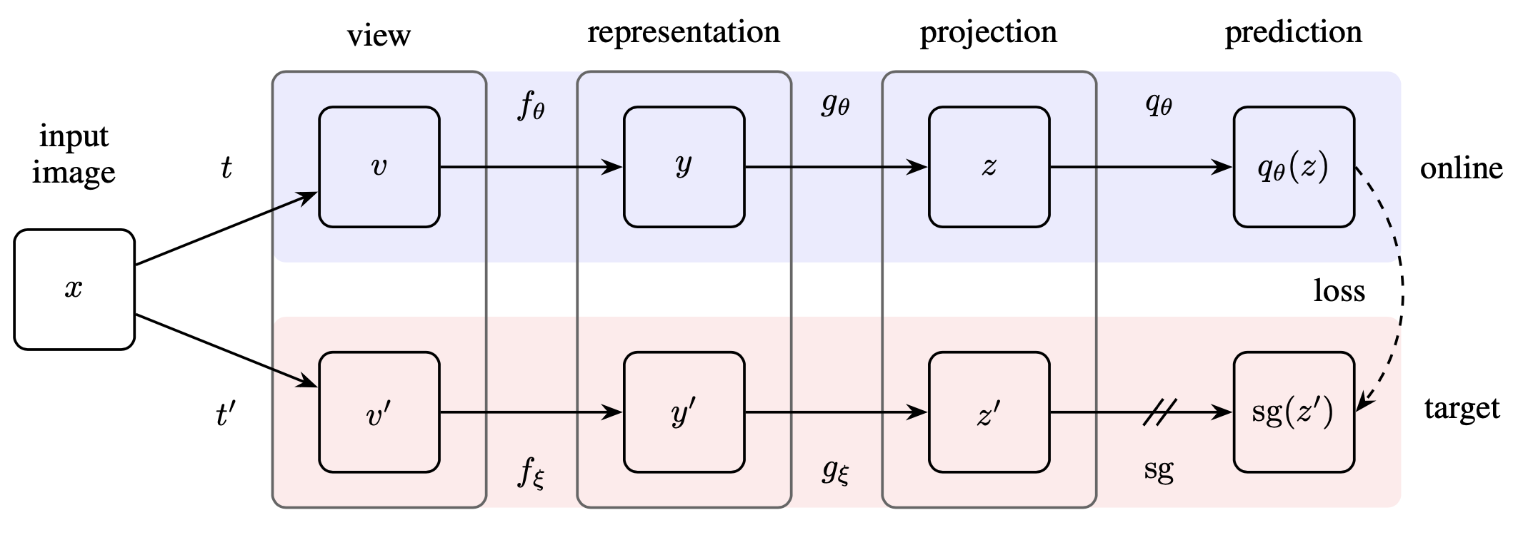
Given an image $\mathbf{x}$, the BYOL loss is constructed as follows:

• Create two augmented views: $\mathbf{v}=t(\mathbf{x}); \mathbf{v}’=t’(\mathbf{x})$, with augmentations sampled $t \sim \mathcal{T}, t’ \sim \mathcal{T}’$;
• Encode them into representations $\mathbf{y}_\theta=f_\theta(\mathbf{v}), \mathbf{y}’=f_\xi(\mathbf{v}’)$;
• Project them into latent variables $\mathbf{z}_\theta=g_\theta(\mathbf{y}_\theta), \mathbf{z}’=g_\xi(\mathbf{y}’)$;
• The online network produces a prediction $q_\theta(\mathbf{z}_\theta)$;
• L2-normalize both $q_\theta(\mathbf{z}_\theta)$ and $\mathbf{z}’$, yielding $\bar{q}_\theta(\mathbf{z}_\theta) = q_\theta(\mathbf{z}_\theta) / | q_\theta(\mathbf{z}_\theta) |$ and $\bar{\mathbf{z}’} = \mathbf{z}’ / |\mathbf{z}’|$;
• Define the loss $\mathcal{L}^\text{BYOL}_\theta$ as the MSE between the L2-normalized prediction $\bar{q}_\theta(\mathbf{z})$ and $\bar{\mathbf{z}’}$;
• Construct the symmetric loss $\tilde{\mathcal{L}}^\text{BYOL}_\theta$ by swapping $\mathbf{v}’$ and $\mathbf{v}$, that is, by feeding $\mathbf{v}’$ to the online network and $\mathbf{v}$ to the target network.
• The final loss is $\mathcal{L}^\text{BYOL}_\theta + \tilde{\mathcal{L}}^\text{BYOL}_\theta$, and only parameters $\theta$ are optimized.

Unlike many widely used contrastive learning approaches, BYOL does not use negative pairs. While most bootstrapping methods depend on pseudo-labels or cluster indices, BYOL directly bootstraps the latent representation.

It is notable, and initially surprising, that BYOL can perform well without negative samples. Later, I came across this post by Abe Fetterman & Josh Albrecht, where they emphasized two unexpected observations from their attempts to reproduce BYOL:

1. BYOL typically performs no better than random when batch normalization is removed.
2. Batch normalization implicitly introduces a form of contrastive learning. They argue that negative samples are important for preventing model collapse (for example, producing an all-zeros representation for every data point). Batch normalization injects dependence on negative samples inexplicitly because, regardless of how similar the inputs in a batch are, the values are re-distributed (spread out $\sim \mathcal{N}(0, 1$). As a result, batch normalization helps prevent collapse. If you work in this area, it is strongly recommended to read the full article.

Memory Bank

Computing embeddings for a large number of negative samples in every batch is extremely expensive. A common alternative is to cache representations in memory, trading off staleness in the stored data for lower computational cost.

Instance Discrimination with Memoy Bank

Instance contrastive learning (Wu et al, 2018) pushes class-based supervision to the extreme by treating each instance as a distinct class of its own. This implies that the number of “classes” equals the number of samples in the training dataset. Training a softmax layer with that many output heads is impractical, but it can be approximated with NCE.

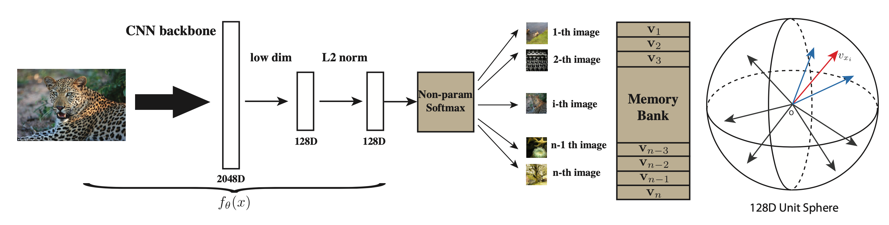
Let $\mathbf{v} = f_\theta(x)$ be the embedding function to learn, and normalize the resulting vector to have $|\mathbf{v}|=1$. A non-parametric classifier predicts the probability that a sample $\mathbf{v}$ belongs to class $i$, using temperature parameter $\tau$:

Rather than recomputing representations for all samples each time, they use a Memory Bank to store sample representations from previous iterations. Let $V=\{ \mathbf{v}_i \}$ denote the memory bank, and let $\mathbf{f}_i = f_\theta(\mathbf{x}_i)$ be the feature produced by forwarding the network. When computing pairwise similarities, we can use the memory-bank representation $\mathbf{v}_i$ instead of the newly computed feature $\mathbf{f}_i$.

In principle, the denominator requires access to the representations of all samples, which is too costly in practice. Instead, it can be estimated with a Monte Carlo approximation using a random subset of $M$ indices $\{j_k\}_{k=1}^M$.

Because there is only one instance per class, training can be unstable and highly variable. To make training smoother, they add an extra positive-sample term to the loss, based on the proximal optimization method. The final NCE loss objective is:

where $\{ \mathbf{v}^{(t-1)} \}$ are embeddings stored in the memory bank from the previous iteration. The difference between iterations $|\mathbf{v}^{(t)}_i - \mathbf{v}^{(t-1)}_i|^2_2$ will gradually vanish as the learned embedding converges.

MoCo & MoCo-V2

Momentum Contrast (MoCo; He et al, 2019) frames unsupervised visual representation learning as a dynamic dictionary look-up. The dictionary is implemented as a large FIFO queue containing encoded representations of data samples.

Given a query sample $\mathbf{x}_q$, we compute a query representation using encoder $\mathbf{q} = f_q(\mathbf{x}_q)$. The dictionary contains key representations $\{\mathbf{k}_1, \mathbf{k}_2, \dots \}$, which are encoded by a momentum encoder $\mathbf{k}_i = f_k (\mathbf{x}^k_i)$. Assume that the dictionary contains exactly one positive key $\mathbf{k}^+$ that matches $\mathbf{q}$. In the paper, $\mathbf{k}^+$ is constructed by taking a noisy copy of $\mathbf{x}_q$ with a different augmentation. The InfoNCE contrastive loss, with temperature $\tau$, is then applied over one positive and $N-1$ negative samples:

Compared to the memory bank approach, MoCo’s queue-based dictionary lets us reuse representations from the most recent mini-batches.

Because the MoCo dictionary is a queue and therefore not differentiable, we cannot update the key encoder $f_k$ via backpropagation through the queue. A naive alternative would be to share the same encoder for both $f_q$ and $f_k$. Instead, MoCo proposes a momentum update with coefficient $m \in [0, 1)$. Let the parameters of $f_q$ and $f_k$ be $\theta_q$ and $\theta_k$, respectively.

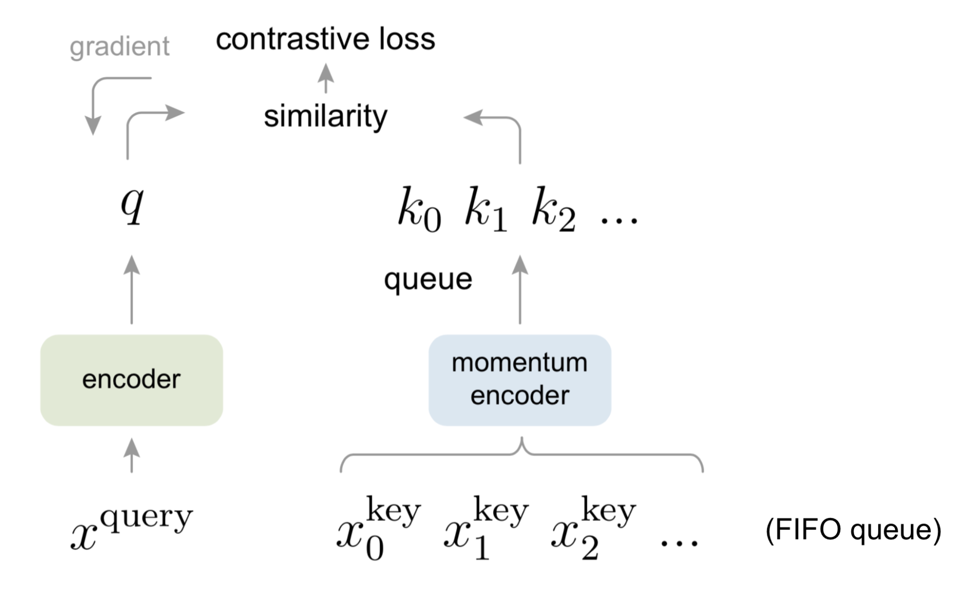
Relative to SimCLR, MoCo’s key advantage is that it decouples batch size from the number of negative samples. In contrast, SimCLR needs a large batch size to obtain enough negatives and suffers performance degradation when the batch size is reduced.

Two SimCLR design choices, namely (1) an MLP projection head and (2) stronger data augmentation, are shown to be highly effective. MoCo V2 (Chen et al, 2020) incorporates both, achieving improved transfer performance without requiring extremely large batch sizes.

CURL

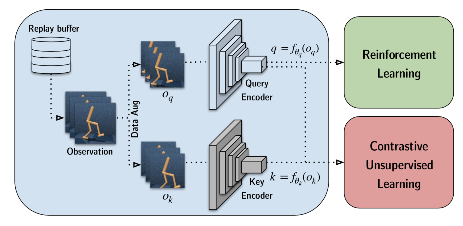
CURL (Srinivas, et al. 2020) applies the ideas above to Reinforcement Learning. It learns a visual representation for RL tasks by matching the embeddings of two augmented versions, $o_q$ and $o_k$, of the raw observation $o$ using a contrastive loss. CURL primarily uses random-crop augmentation. As in MoCo, the key encoder is implemented as a momentum encoder whose weights are an EMA of the query encoder weights.

A key difference between RL and supervised visual tasks is that RL relies on temporal consistency across consecutive frames. Accordingly, CURL applies augmentation consistently to each frame stack so that information about the temporal structure of the observation is preserved.

Feature Clustering

DeepCluster

DeepCluster (Caron et al. 2018) alternates between clustering features using k-means and treating the resulting cluster assignments as pseudo-labels to provide supervised training signals.

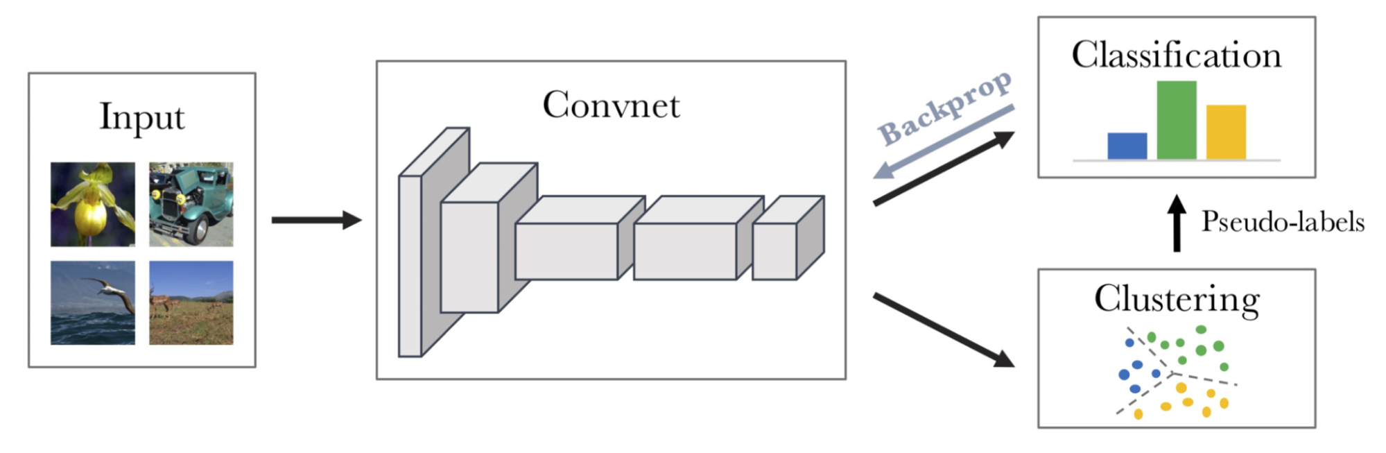
At each iteration, DeepCluster clusters data points using the current representation, then uses the new cluster assignments as classification targets to learn an updated representation. However, this alternating procedure is susceptible to trivial solutions. Although it avoids negative pairs, it requires an expensive clustering stage and additional precautions to prevent collapse to trivial outcomes.

SwAV

SwAV (Swapping Assignments between multiple Views; Caron et al. 2020) is an online contrastive learning algorithm. It computes a code from one augmented view of an image and trains the model to predict that code from another augmented view of the same image.

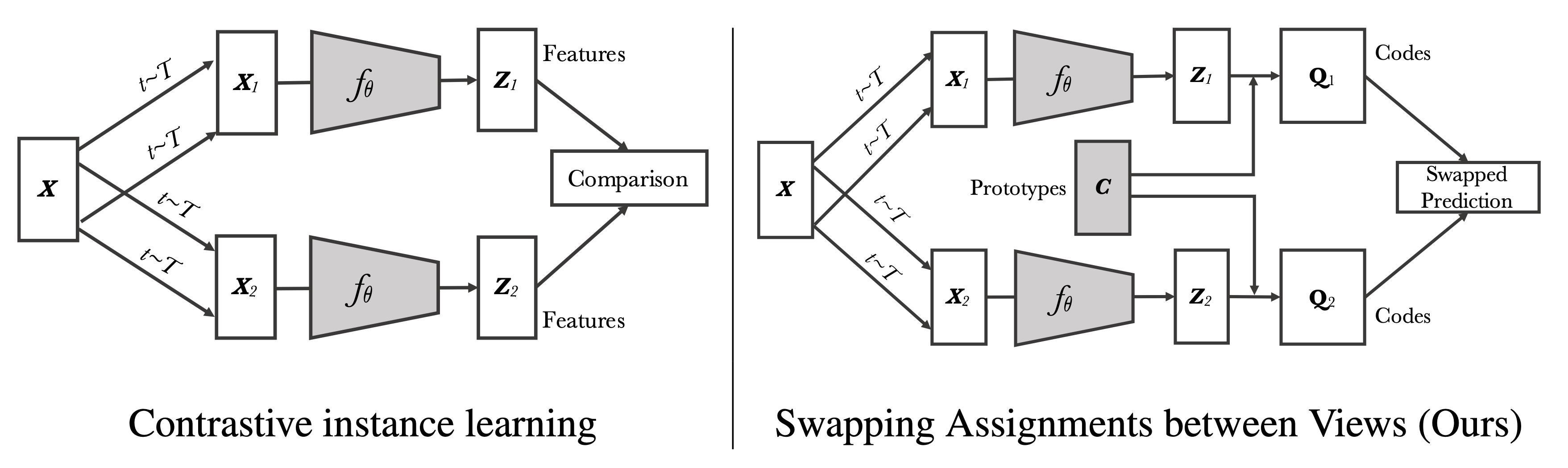
Given image features under two different augmentations, $\mathbf{z}_t$ and $\mathbf{z}_s$, SwAV computes the corresponding codes $\mathbf{q}_t$ and $\mathbf{q}_s$. The loss evaluates the fit by swapping the two codes, using $\ell(.)$ to measure the fit between a feature and a code.

The swapped-fit prediction is based on cross entropy between the predicted code and a set of $K$ trainable prototype vectors $\mathbf{C} = \{\mathbf{c}_1, \dots, \mathbf{c}_K\}$. The prototype matrix is shared across batches and represents anchor clusters to which each instance should be assigned.

For a mini-batch containing $B$ feature vectors $\mathbf{Z} = [\mathbf{z}_1, \dots, \mathbf{z}_B]$, define the mapping matrix between features and prototypes as $\mathbf{Q} = [\mathbf{q}_1, \dots, \mathbf{q}_B] \in \mathbb{R}_+^{K\times B}$. The objective is to maximize similarity between features and prototypes:

where $\mathcal{H}$ is the entropy, $\mathcal{H}(\mathbf{Q}) = - \sum_{ij} \mathbf{Q}_{ij} \log \mathbf{Q}_{ij}$, which controls code smoothness. The coefficient $\epsilon$ must not be too large, otherwise all samples are assigned uniformly across all clusters. The feasible solution set for $\mathbf{Q}$ requires each mapping matrix to have rows summing to $1/K$ and columns summing to $1/B$, which enforces that each prototype is selected at least $B/K$ times on average.

SwAV uses the iterative Sinkhorn-Knopp algorithm (Cuturi 2013) to solve for $\mathbf{Q}$.

Working with Supervised Datasets

CLIP

CLIP (Contrastive Language-Image Pre-training; Radford et al. 2021) jointly trains a text encoder and an image feature extractor on a pretraining task that predicts which caption corresponds to which image.

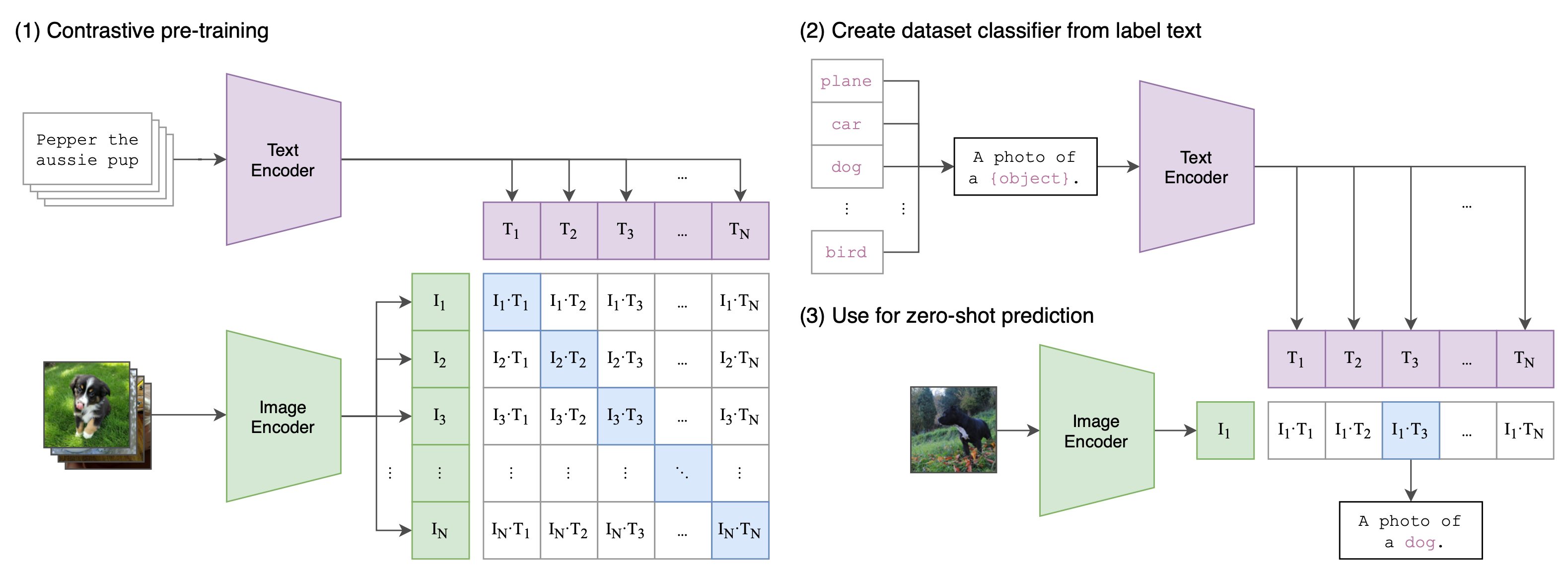
Given a batch of $N$ (image, text) pairs, CLIP computes a dense cosine similarity matrix over all $N\times N$ possible (image, text) candidates in the batch. The text and image encoders are trained jointly to maximize similarity for the $N$ correct (image, text) pairings while minimizing similarity for the $N(N-1)$ incorrect pairings, using a symmetric cross entropy loss over the dense matrix.

See the numy-like pseudo code for CLIP in

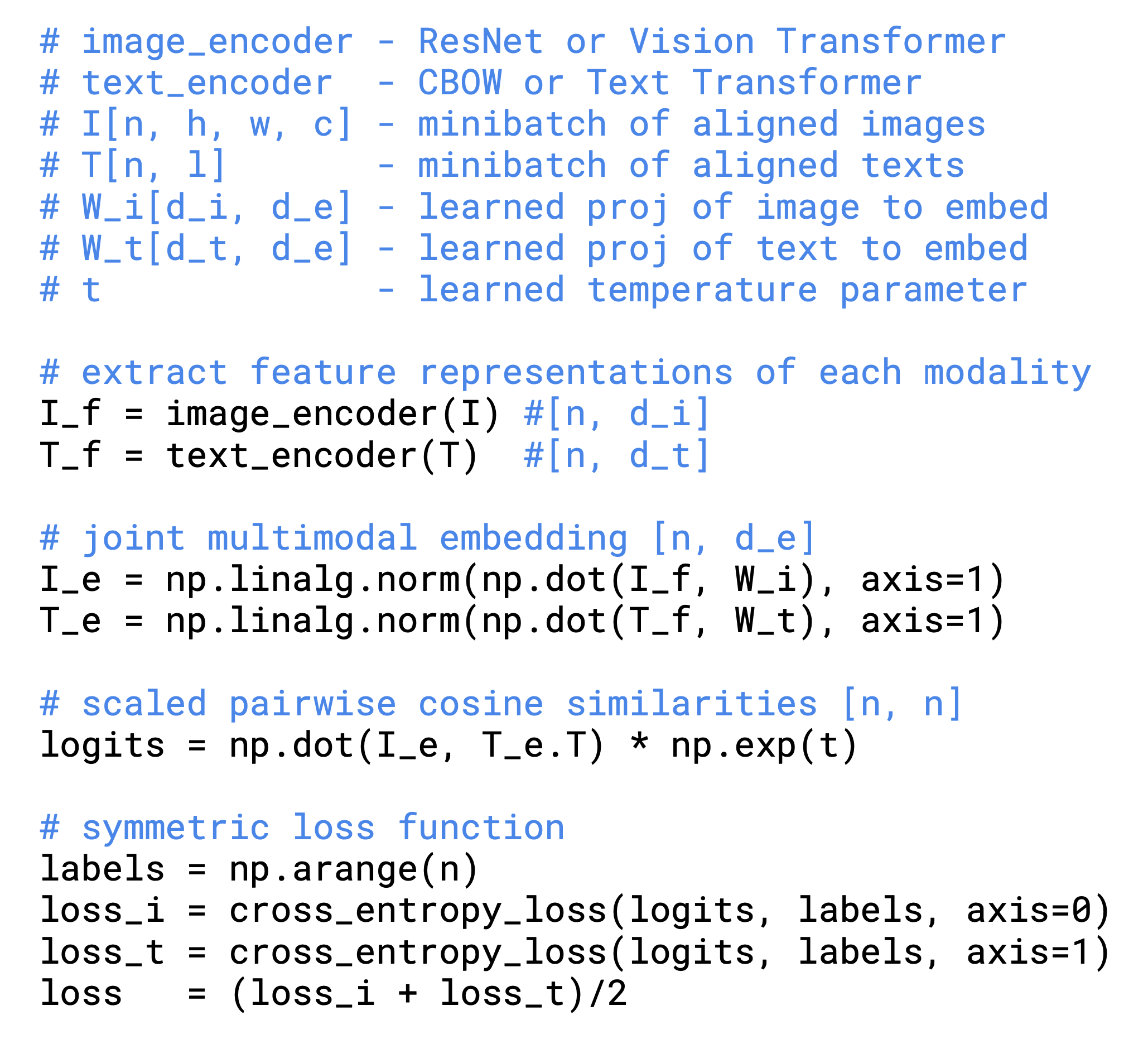
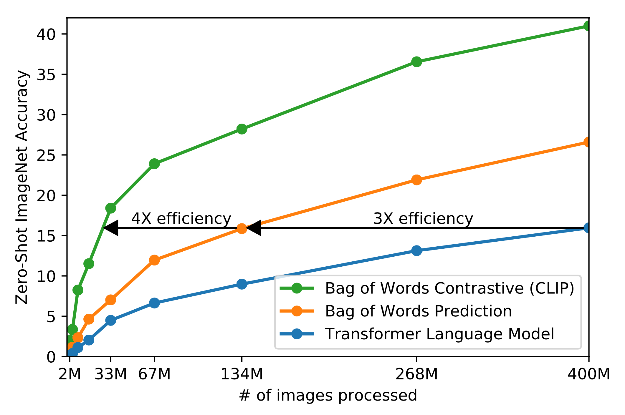
Relative to the other methods above for learning strong visual representations, what makes CLIP distinctive is “the appreciation of using natural language as a training signal”. It requires access to a supervised dataset where the text-image correspondence is known. CLIP is trained on 400 million (text, image) pairs collected from the Internet. The query list includes all words that occur at least 100 times in the English version of Wikipedia. Notably, the authors report that Transformer-based language models are 3x slower than a bag-of-words (BoW) text encoder for zero-shot ImageNet classification. They also find that using a contrastive objective, rather than predicting the exact words associated with images (as is common in image captioning), improves data efficiency by another 4x.

CLIP produces visual representations that transfer non-trivially to many CV benchmark datasets, with results competitive with supervised baselines. Across the tested transfer tasks, CLIP struggles with very fine-grained classification and with abstract or systematic tasks such as counting objects. CLIP transfer performance correlates smoothly with the amount of model compute.

Supervised Contrastive Learning

Cross entropy loss is known to have several issues, including limited robustness to noisy labels and potentially poor margins. Common improvements typically focus on curating better training data, for example through label smoothing and data augmentation. Supervised Contrastive Loss (Khosla et al. 2021) aims to use label information more effectively than cross entropy by enforcing that normalized embeddings from the same class are closer than embeddings from different classes.

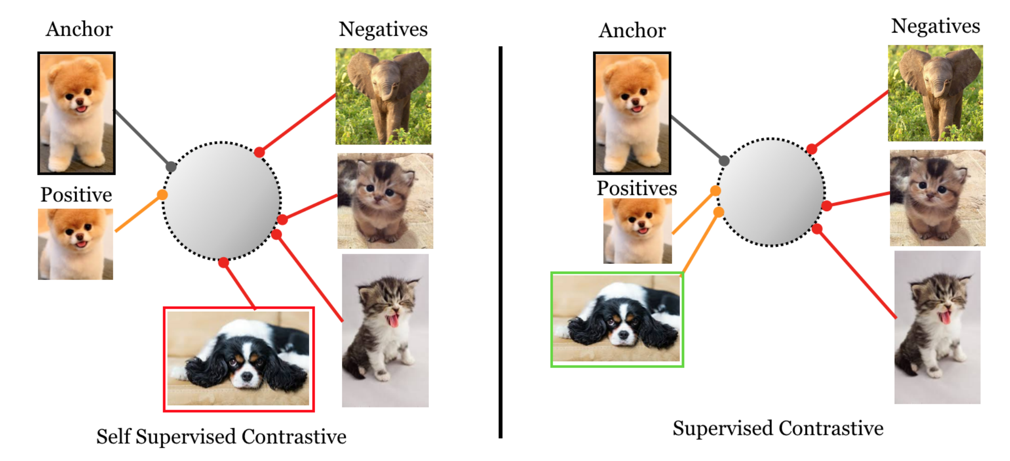
Given a randomly sampled set of $n$ (image, label) pairs, $\{\mathbf{x}_i, y_i\}_{i=1}^n$, we can create $2n$ training pairs by applying two random augmentations to each sample, $\{\tilde{\mathbf{x}}_i, \tilde{y}_i\}_{i=1}^{2n}$.

The supervised contrastive loss $\mathcal{L}_\text{supcon}$ uses multiple positive and negative samples and is closely related to soft nearest-neighbor loss:

where $\mathbf{z}_k=P(E(\tilde{\mathbf{x}_k}))$, in which $E(.)$ is an encoder network (mapping an augmented image to a vector) and $P(.)$ is a projection network (mapping one vector to another). $N_i= \{j \in I: \tilde{y}_j = \tilde{y}_i \}$ denotes the set of indices for samples with label $y_i$. Expanding the positive set $N_i$ leads to improved results.

Based on their experiments, supervised contrastive loss:

• outperforms standard cross entropy, although only by a small margin.
• outperforms cross entropy on robustness benchmarks (ImageNet-C, which applies common naturally occuring perturbations such as noise, blur and contrast changes to the ImageNet dataset).
• is less sensitive to hyperparameter variations.

Language: Sentence Embedding

This section explains approaches for learning sentence embeddings.

Text Augmentation

In computer vision, most contrastive learning methods rely on generating an augmented view of each image. For text, producing augmentations is more difficult because edits can easily change a sentence’s meaning. Here, we examine three augmentation families for text sequences: lexical edits, back-translation, and cutoff or dropout based perturbations.

Lexical Edits

EDA (Easy Data Augmentation; Wei & Zou 2019) introduces a small set of simple yet effective augmentation operations. Given an input sentence, EDA randomly selects and applies one of four operations:

1. Synonym replacement (SR): Replace $n$ randomly selected non-stop words with their synonyms.
2. Random insertion (RI): Insert a random synonym of a randomly chosen non-stop word at a random position in the sentence.
3. Random swap (RS): Randomly swap two words, repeating the swap $n$ times.
4. Random deletion (RD): Independently delete each word in the sentence with probability $p$.

where $p=\alpha$ and $n=\alpha \times \text{sentence_length}$, motivated by the intuition that longer sentences can tolerate more noise while still preserving the original label. The hyperparameter $\alpha$ roughly specifies what fraction of the words in a sentence may be modified by a single augmentation.

EDA is reported to improve classification accuracy across several benchmark text classification datasets relative to a baseline without EDA. The gain is larger when the training set is smaller. All four EDA operations contribute to accuracy improvements, although they reach their best performance at different values of $\alpha$.

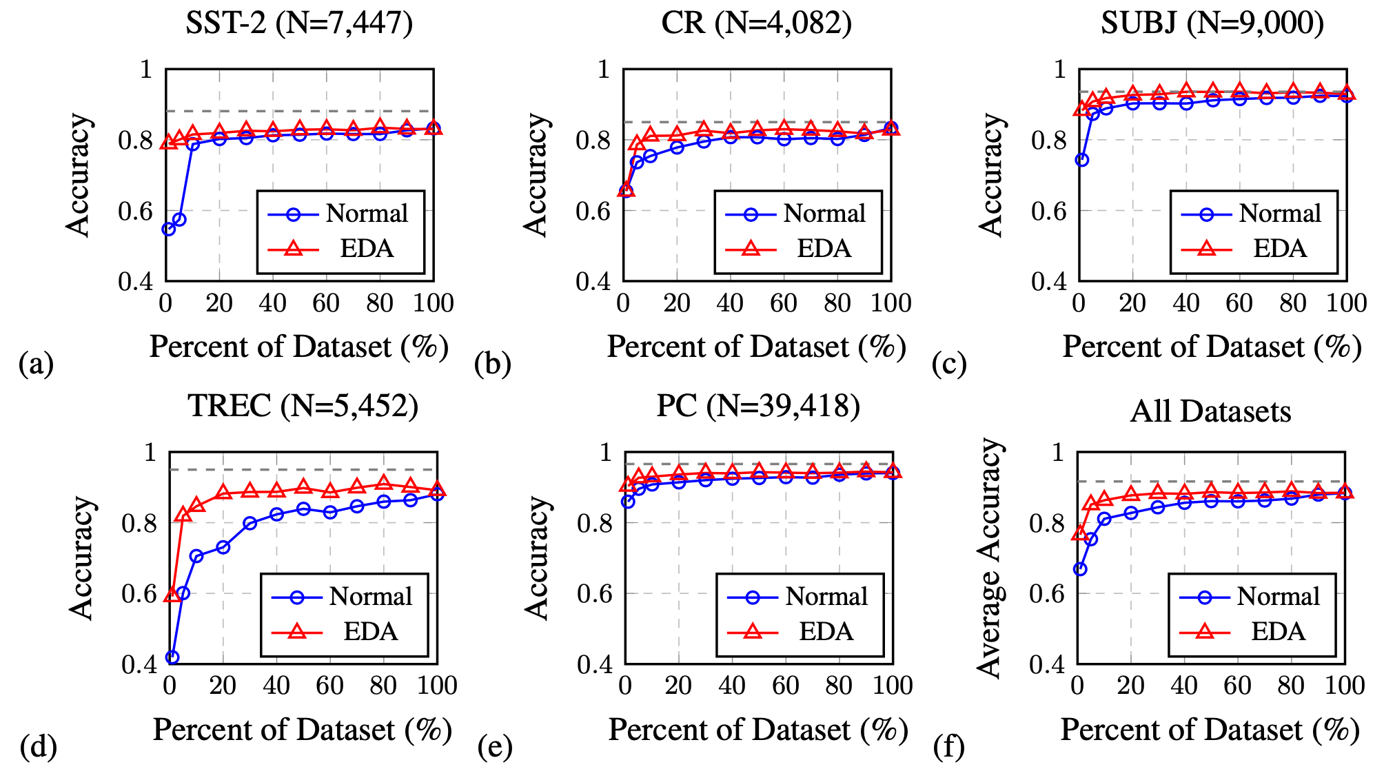
In Contextual Augmentation (Sosuke Kobayashi, 2018), a replacement for word $w_i$ at position $i$ is sampled from a probability distribution $p(.\mid S\setminus\{w_i\})$, predicted by a bidirectional language model such as BERT, enabling fluent context-aware substitutions.

Back-translation

CERT (Contrastive self-supervised Encoder Representations from Transformers; Fang et al. (2020); code) creates augmented sentences through back-translation. Different translation models across languages can be used to generate multiple augmented variants. After producing noisy versions of text samples, previously described contrastive learning frameworks (for example, MoCo) can be applied to learn sentence embeddings.

Dropout and Cutoff

Shen et al. (2020) introduced Cutoff as a text augmentation technique, drawing inspiration from cross-view training. They described three cutoff augmentation strategies:

1. Token cutoff removes the information from a small set of selected tokens. To avoid data leakage, the corresponding entries in the input embeddings, positional embeddings, and any other relevant embedding matrices should all be set to zero.,
2. Feature cutoff removes a small number of feature columns.
3. Span cutoff removes a contiguous span of text.

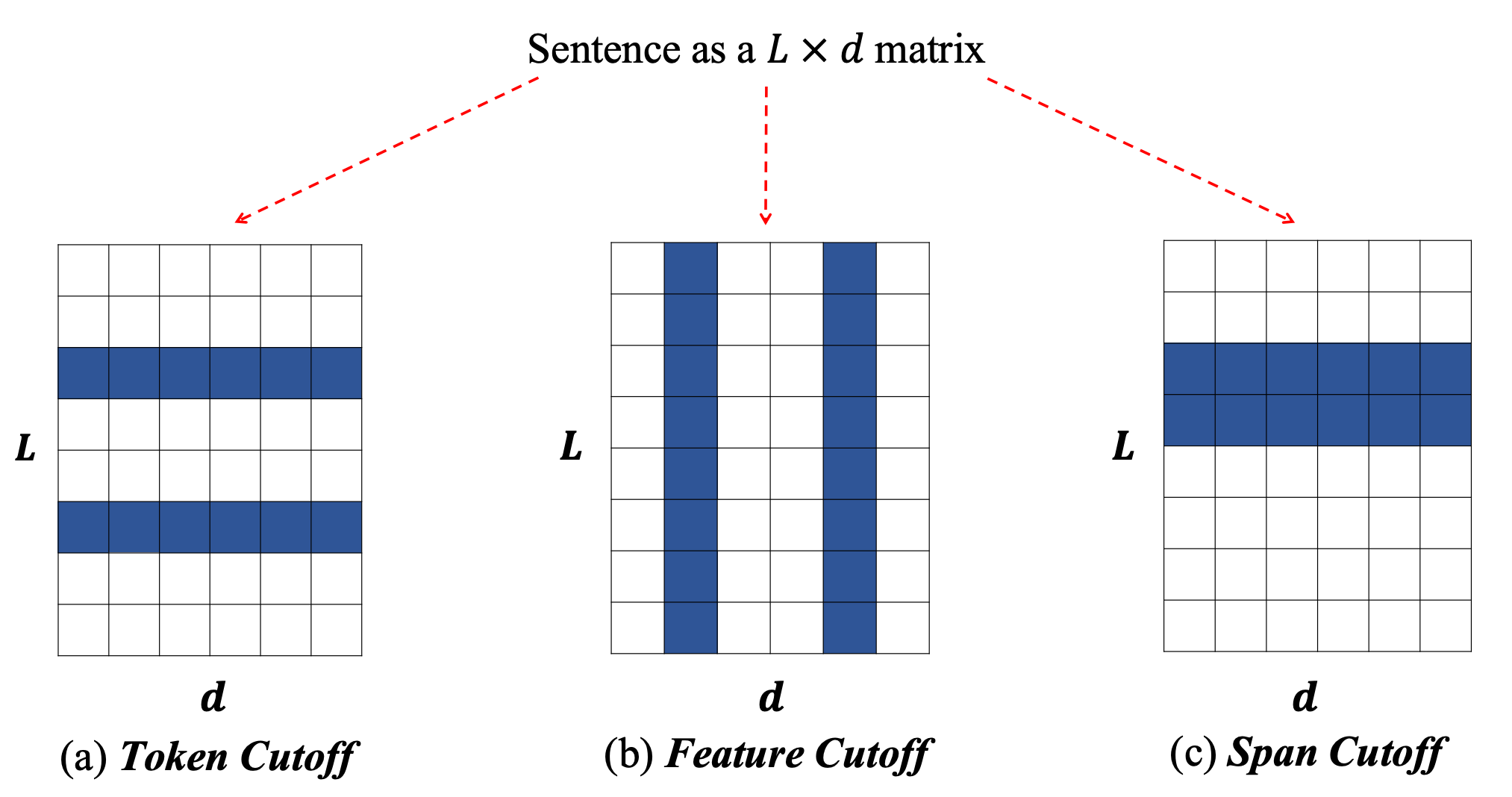
It is possible to generate multiple augmented variants of a single sample. During training, Shen et al. (2020) added a KL-divergence term to quantify agreement between predictions produced from different augmented versions.

SimCSE (Gao et al. 2021; code) trains on unsupervised data by predicting a sentence from itself using only dropout as noise. That is, dropout functions as the data augmentation mechanism for text sequences. The same sample is passed through the encoder twice using different dropout masks, forming a positive pair, while other in-batch samples serve as negative pairs. This resembles cutoff-based augmentation, but dropout is more flexible, with less explicit semantics for which content is masked.

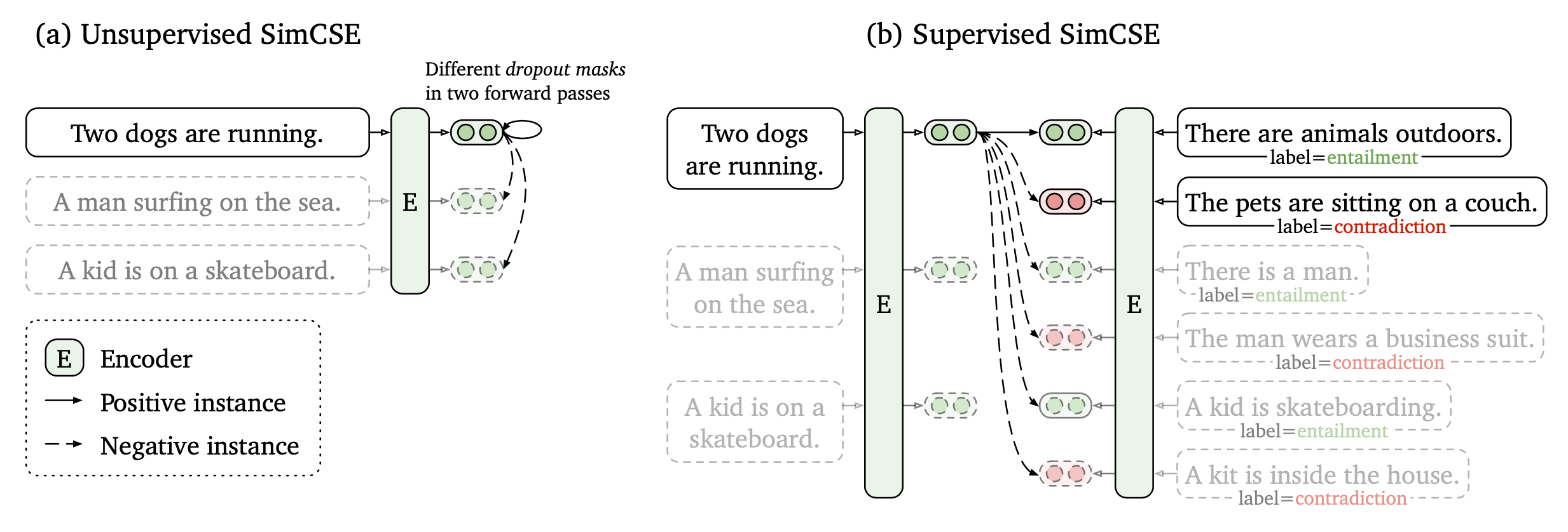
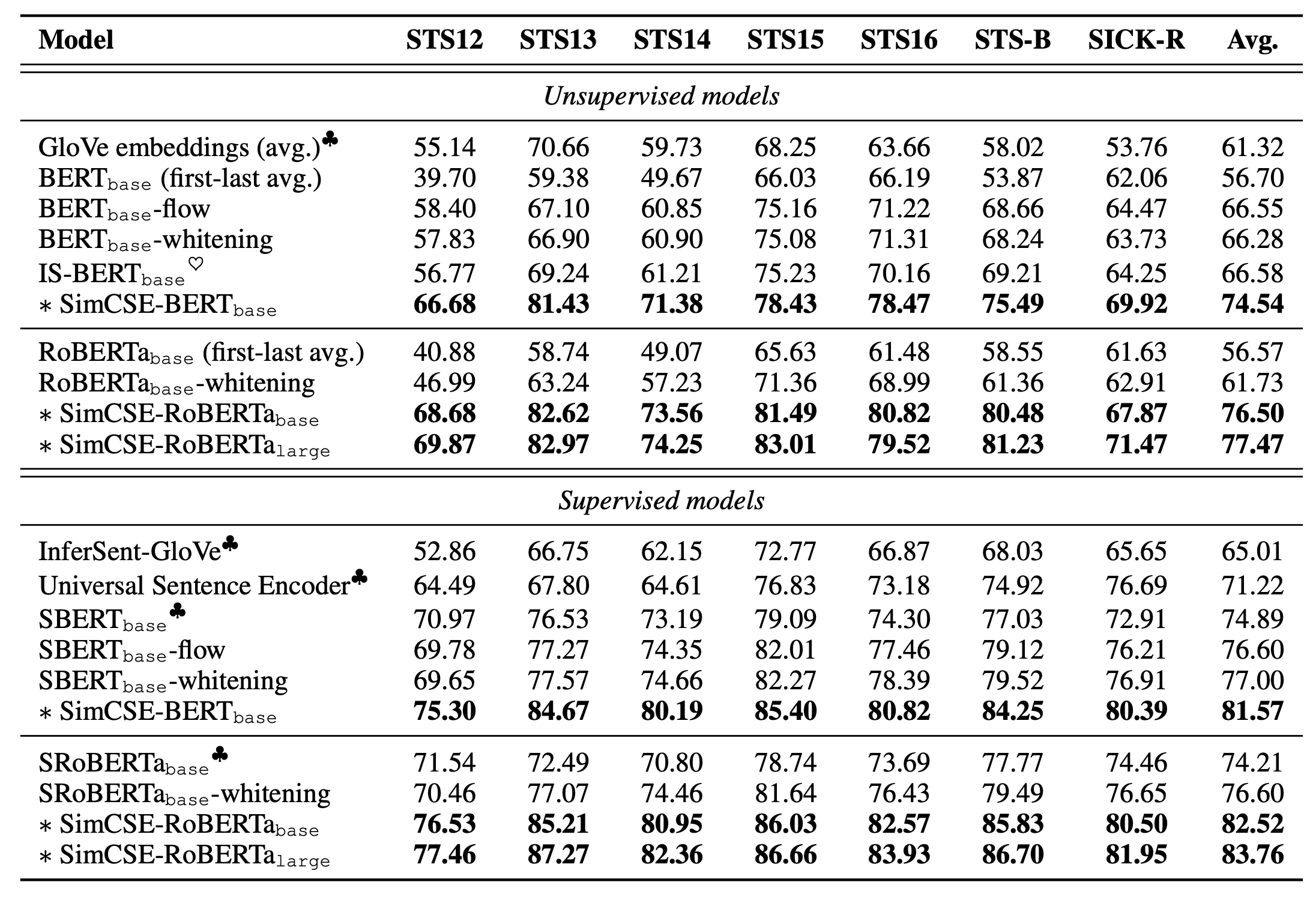
They evaluated on 7 STS (Semantic Text Similarity) datasets by computing cosine similarity between sentence embeddings. They also explored an optional MLM auxiliary objective loss intended to mitigate catastrophic forgetting of token-level knowledge. This auxiliary loss improved performance on transfer tasks but caused a consistent decline on the main STS tasks.

Supervision from NLI

Empirical results indicate that sentence embeddings taken directly from a pre-trained BERT model, without fine-tuning, perform poorly on semantic similarity tasks. Rather than using these raw representations, the embeddings typically need further refinement via fine-tuning.

Natural Language Inference (NLI) tasks are a primary source of supervised training signals for sentence embedding learning, including datasets such as SNLI, MNLI, and QQP.

Sentence-BERT

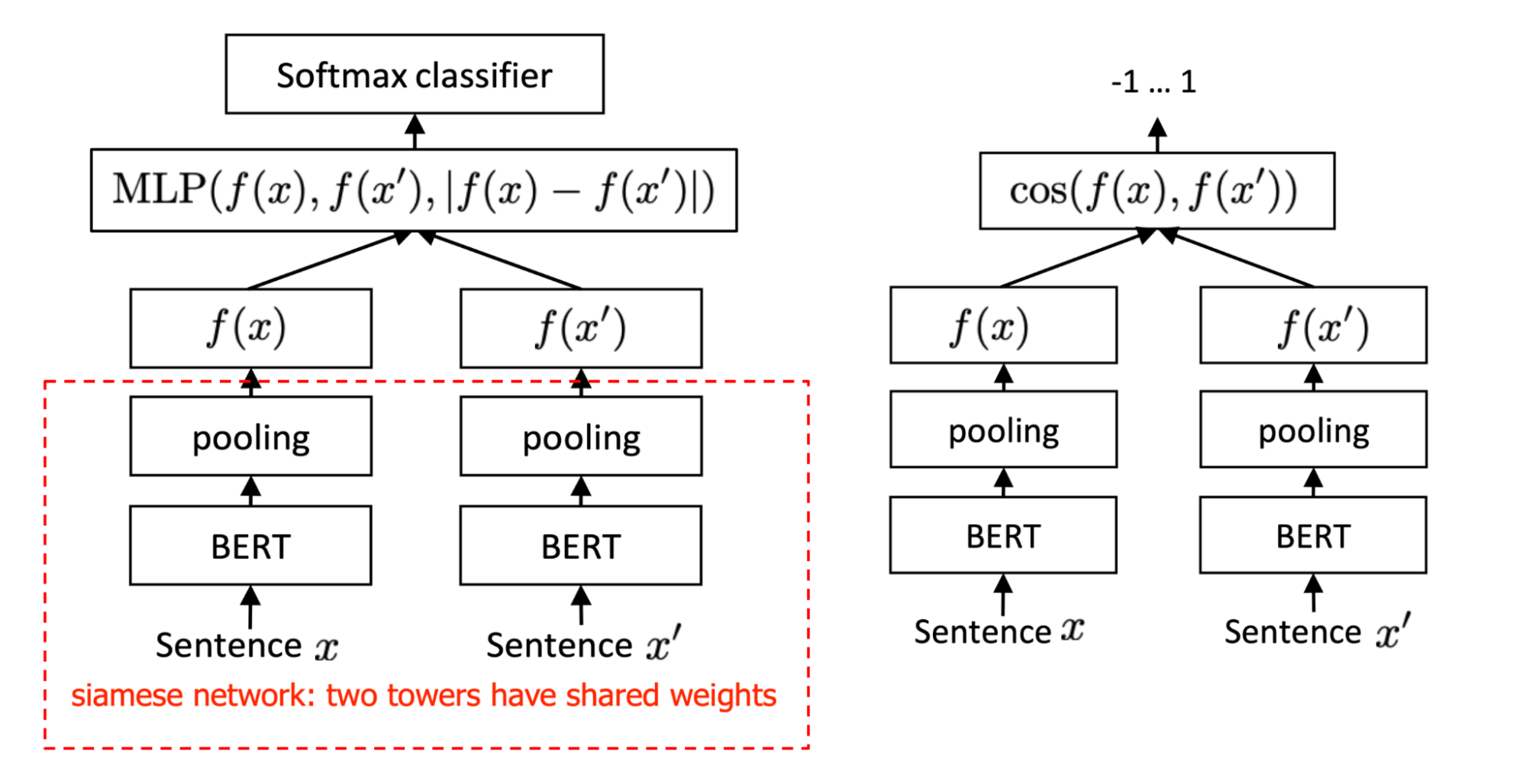
SBERT (Sentence-BERT) (Reimers & Gurevych, 2019) uses siamese and triplet network architectures to learn sentence embeddings so that sentence similarity can be computed as the cosine similarity between embedding pairs. SBERT training depends on supervised data, because the model is fine-tuned on multiple NLI datasets.

They evaluated several prediction heads added on top of the BERT encoder:

• Softmax classification objective: The siamese network’s classification head is built from the concatenation of two embeddings $f(\mathbf{x}), f(\mathbf{x}’)$ and $\vert f(\mathbf{x}) - f(\mathbf{x}’) \vert$. The predicted output is $\hat{y}=\text{softmax}(\mathbf{W}_t [f(\mathbf{x}); f(\mathbf{x}’); \vert f(\mathbf{x}) - f(\mathbf{x}’) \vert])$. They reported that the most critical component is the element-wise difference $\vert f(\mathbf{x}) - f(\mathbf{x}’) \vert$.
• Regression objective: This uses a regression loss on $\cos(f(\mathbf{x}), f(\mathbf{x}’))$, where the pooling strategy has a substantial effect. In experiments, max pooling performed much worse than mean pooling and the CLS-token representation.
• Triplet objective: $\max(0, |f(\mathbf{x}) - f(\mathbf{x}^+)|- |f(\mathbf{x}) - f(\mathbf{x}^-)| + \epsilon)$, where $\mathbf{x}, \mathbf{x}^+, \mathbf{x}^-$ are the embeddings for the anchor, positive, and negative sentences.

Across datasets, the best-performing objective function varies, so no single objective is universally optimal.

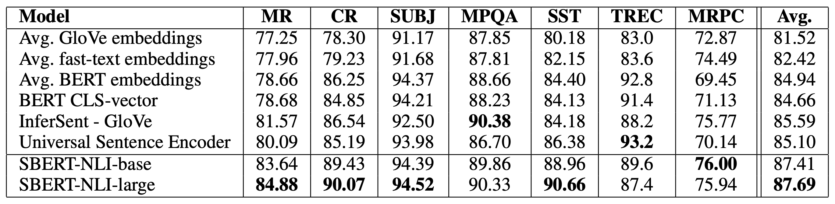
The SentEval library (Conneau and Kiela, 2018) is widely used to evaluate the quality of learned sentence embeddings. SBERT exceeded other contemporaneous baselines (Aug 2019) on 5 of the 7 SentEval tasks.

BERT-flow

An embedding space is considered isotropic when embeddings are distributed uniformly across each dimension; if not, the space is anisotropic. Li et al, (2020) reported that a pre-trained BERT model yields a non-smooth, anisotropic semantic space for sentence embeddings, which contributes to poor performance on text similarity tasks in the absence of fine-tuning. Empirically, they highlighted two issues affecting BERT sentence embeddings: Word frequency distorts the embedding space. High-frequency words lie closer to the origin, whereas low-frequency words are farther from the origin. Low-frequency words are distributed more sparsely. Embeddings for low-frequency words tend to be farther from their $k$-NN neighbors, while high-frequency word embeddings are more densely concentrated.

BERT-flow (Li et al, 2020; code) was introduced to calibrate embeddings by mapping them to a smooth, isotropic Gaussian distribution using normalizing flows.

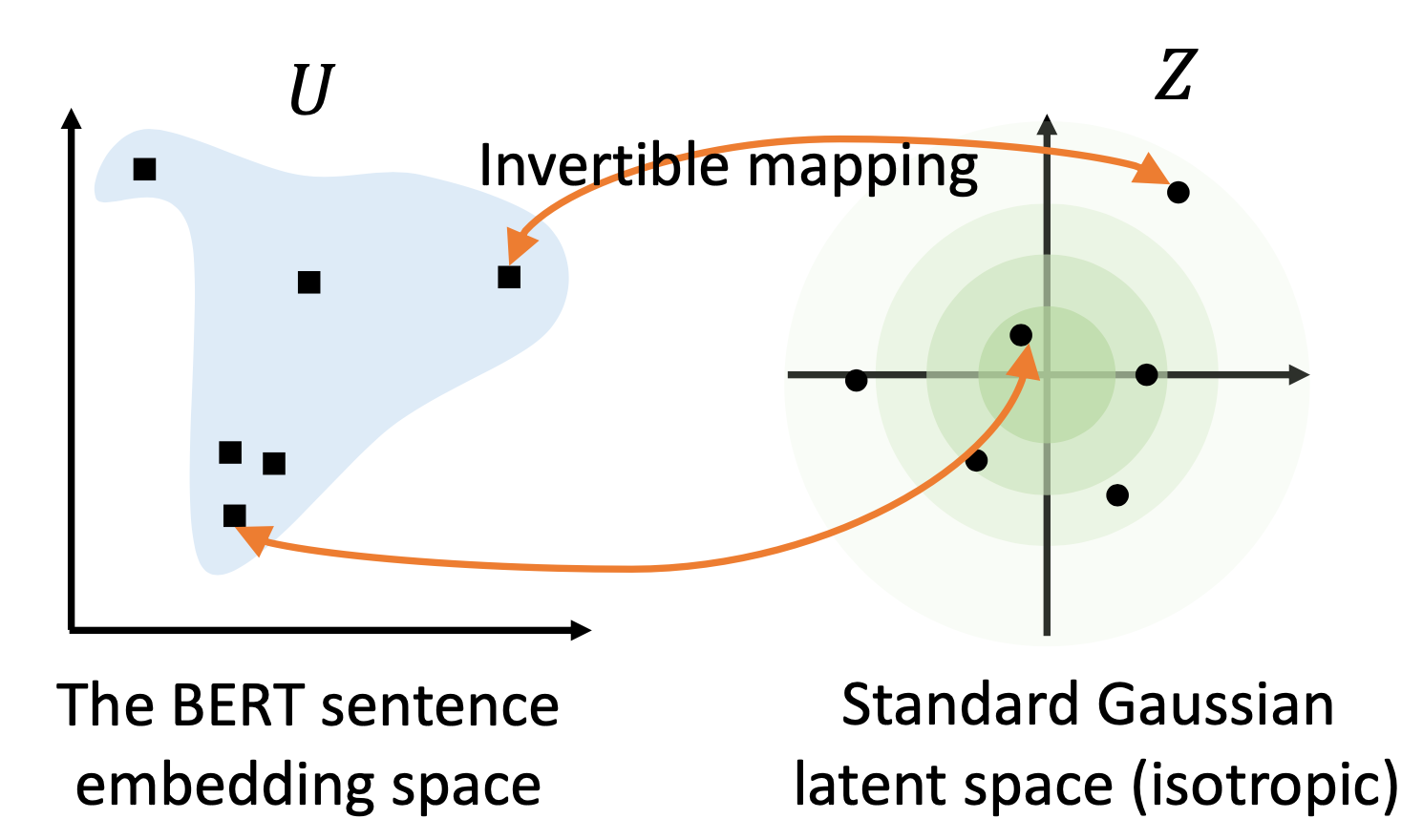
Let $\mathcal{U}$ denote the observed BERT sentence embedding space, and let $\mathcal{Z}$ denote the target latent space, a standard Gaussian. Accordingly, $p_\mathcal{Z}$ is a Gaussian density function, and $f_\phi: \mathcal{Z}\to\mathcal{U}$ is an invertible transformation:

A flow-based generative model learns this invertible mapping by maximizing the likelihood of the marginal distribution of $\mathcal{U}$:

where $s$ is a sentence sampled from the text corpus $\mathcal{D}$. Only the flow parameters $\phi$ are optimized; the parameters of the pretrained BERT model remain fixed.

BERT-flow was shown to improve performance on most STS tasks, both with and without supervision from NLI datasets. Because normalizing-flow calibration does not require labels, it can be trained using the full dataset, including validation and test sets.

Whitening Operation

Su et al. (2021) applied a whitening operation to improve the isotropy of learned representations and to reduce sentence embedding dimensionality.

This method shifts sentence vectors to have mean 0 and transforms their covariance matrix to the identity. Given a set of samples $\{\mathbf{x}_i\}_{i=1}^N$, let $\tilde{\mathbf{x}}_i$ denote the transformed samples and $\tilde{\Sigma}$ the corresponding covariance matrix:

Applying SVD to $\Sigma = U\Lambda U^\top$ yields $W^{-1}=\sqrt{\Lambda} U^\top$ and $W=U\sqrt{\Lambda^{-1}}$. Within the SVD, $U$ is an orthogonal matrix whose columns are eigenvectors, and $\Lambda$ is a diagonal matrix with positive entries representing the eigenvalues in sorted order.

Dimensionality reduction can be performed by retaining only the first $k$ columns of $W$, referred to as Whitening-$k$.

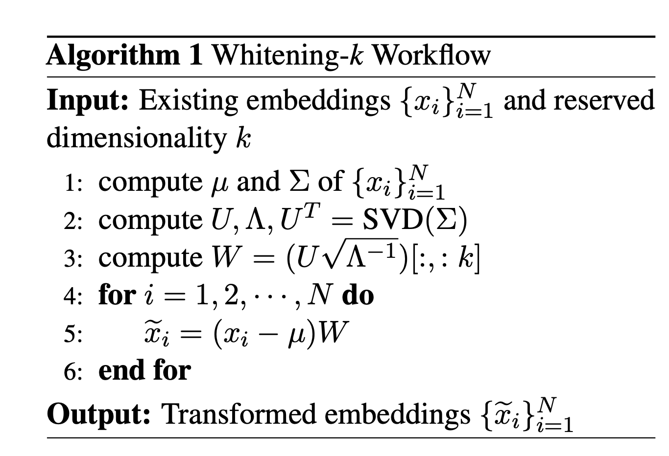
Whitening was reported to outperform BERT-flow and to achieve SOTA on many STS benchmarks with 256-dimensional sentence embeddings, both with and without NLI supervision.

Unsupervised Sentence Embedding Learning

Context Prediction

Quick-Thought (QT) vectors (Logeswaran & Lee, 2018) cast sentence representation learning as a classification problem: given a sentence and its surrounding context, a classifier separates true context sentences from contrastive alternatives using their vector representations (the “cloze test”). This setup removes the softmax output layer that can slow training.

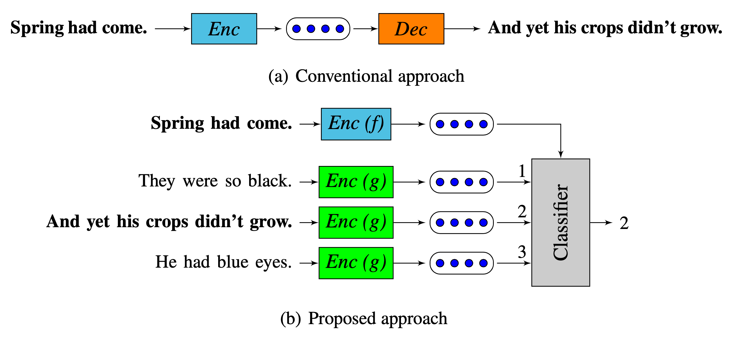
Let $f(.)$ and $g(.)$ be two encoding functions that map a sentence $s$ to a fixed-length vector. Let $C(s)$ be the set of sentences in the context of $s$, and let $S(s)$ be the candidate set that contains exactly one true context sentence $s_c \in C(s)$ along with many non-context negative sentences. The Quick-Thought model is trained to maximize the probability of selecting the single correct context sentence $s_c \in S(s)$. This is effectively an NCE loss when treating the sentence pair $(s, s_c)$ as positive and all other pairs $(s, s’)$, where $s’ \in S(s), s’\neq s_c$, as negatives.

Mutual Information Maximization

IS-BERT (Info-Sentence BERT) (Zhang et al. 2020; code) uses a self-supervised objective based on mutual information maximization to learn high-quality sentence embeddings in an unsupervised setting.

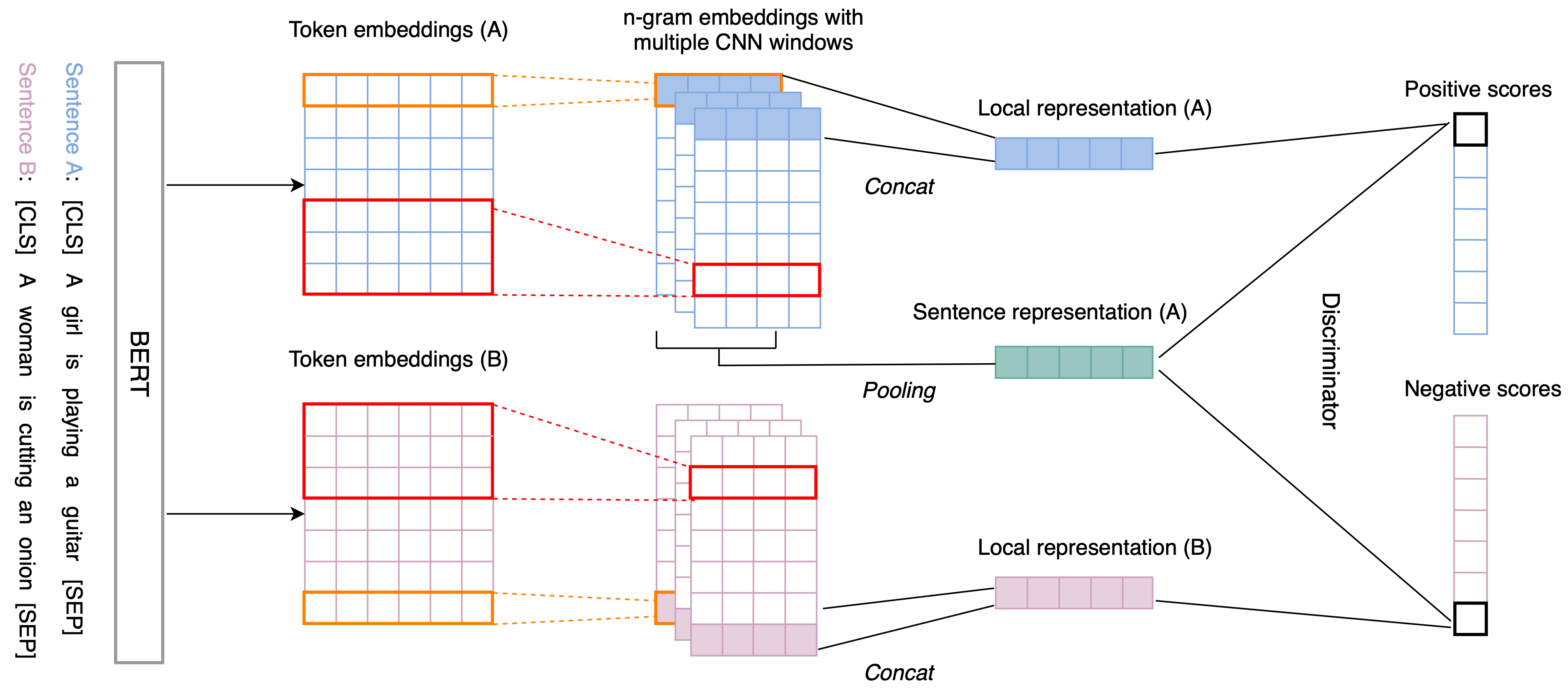
IS-BERT proceeds as follows:

1. Encode an input sentence $s$ with BERT to obtain a token embedding sequence of length $l$, $\mathbf{h}_{1:l}$.

2. Apply a 1-D convolutional network with multiple kernel sizes (for example, 1, 3, 5) over the token embedding sequence to capture local n-gram dependencies: $\mathbf{c}_i = \text{ReLU}(\mathbf{w} \cdot \mathbf{h}_{i:i+k-1} + \mathbf{b})$. The resulting sequences are padded to match the input length.

3. Construct the final local representation for the $i$-th token $\mathcal{F}_\theta^{(i)} (\mathbf{x})$ by concatenating the representations produced by the different kernel sizes.

4. Compute the global sentence representation $\mathcal{E}_\theta(\mathbf{x})$ by applying mean-over-time pooling to the token representations $\mathcal{F}_\theta(\mathbf{x}) = \{\mathcal{F}_\theta^{(i)} (\mathbf{x}) \in \mathbb{R}^d\}_{i=1}^l$.

Because mutual information estimation is generally intractable for continuous, high-dimensional random variables, IS-BERT adopts the Jensen-Shannon estimator (Nowozin et al., 2016, Hjelm et al., 2019) to maximize the mutual information between $\mathcal{E}_\theta(\mathbf{x})$ and $\mathcal{F}_\theta^{(i)} (\mathbf{x})$.

where $T_\omega: \mathcal{F}\times\mathcal{E} \to \mathbb{R}$ is a learnable network with parameters $\omega$ that produces discriminator scores. The negative sample $\mathbf{x}’$ is drawn from the distribution $\tilde{P}=P$. $\text{sp}(x)=\log(1+e^x)$ denotes the softplus activation function.

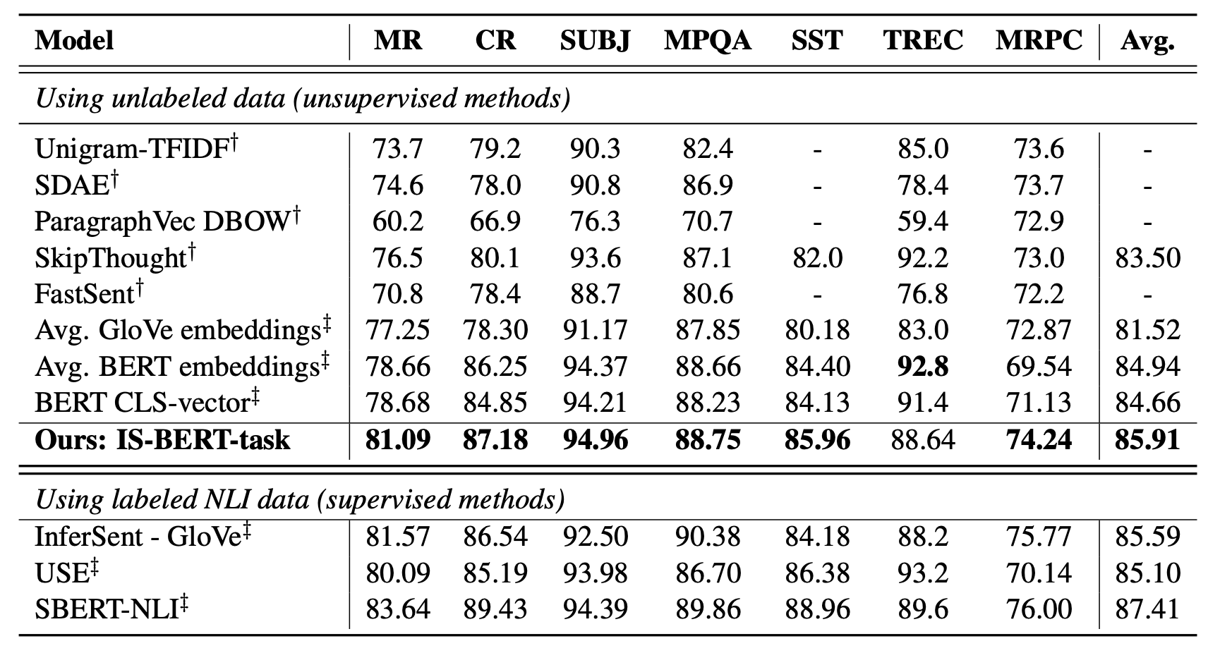
On SentEval, IS-BERT’s unsupervised results outperformed most unsupervised baselines (Sep 2020), though they were, as expected, weaker than supervised settings. With labeled NLI datasets, IS-BERT achieved results comparable to SBERT (See Fig. 25 & 30).

Citation

Cited as:

Weng, Lilian. (May 2021). Contrastive representation learning. Lil’Log. https://lilianweng.github.io/posts/2021-05-31-contrastive/.

Or

@article{weng2021contrastive,
  title   = "Contrastive Representation Learning",
  author  = "Weng, Lilian",
  journal = "lilianweng.github.io",
  year    = "2021",
  month   = "May",
  url     = "https://lilianweng.github.io/posts/2021-05-31-contrastive/"
}

References

[1] Sumit Chopra, Raia Hadsell and Yann LeCun. “Learning a similarity metric discriminatively, with application to face verification.” CVPR 2005.

[2] Florian Schroff, Dmitry Kalenichenko and James Philbin. “FaceNet: A Unified Embedding for Face Recognition and Clustering.” CVPR 2015.

[3] Hyun Oh Song et al. “Deep Metric Learning via Lifted Structured Feature Embedding.” CVPR 2016. [code]

[4] Ruslan Salakhutdinov and Geoff Hinton. “Learning a Nonlinear Embedding by Preserving Class Neighbourhood Structure” AISTATS 2007.

[5] Michael Gutmann and Aapo Hyvärinen. “Noise-contrastive estimation: A new estimation principle for unnormalized statistical models.” AISTATS 2010.

[6] Kihyuk Sohn et al. “Improved Deep Metric Learning with Multi-class N-pair Loss Objective” NIPS 2016.

[7] Nicholas Frosst, Nicolas Papernot and Geoffrey Hinton. “Analyzing and Improving Representations with the Soft Nearest Neighbor Loss.” ICML 2019

[8] Tongzhou Wang and Phillip Isola. “Understanding Contrastive Representation Learning through Alignment and Uniformity on the Hypersphere.” ICML 2020. [code]

[9] Zhirong Wu et al. “Unsupervised feature learning via non-parametric instance-level discrimination.” CVPR 2018.

[10] Ekin D. Cubuk et al. “AutoAugment: Learning augmentation policies from data.” arXiv preprint arXiv:1805.09501 (2018).

[11] Daniel Ho et al. “Population Based Augmentation: Efficient Learning of Augmentation Policy Schedules.” ICML 2019.

[12] Ekin D. Cubuk & Barret Zoph et al. “RandAugment: Practical automated data augmentation with a reduced search space.” arXiv preprint arXiv:1909.13719 (2019).

[13] Hongyi Zhang et al. “mixup: Beyond Empirical Risk Minimization.” ICLR 2017.

[14] Sangdoo Yun et al. “CutMix: Regularization Strategy to Train Strong Classifiers with Localizable Features.” ICCV 2019.

[15] Yannis Kalantidis et al. “Mixing of Contrastive Hard Negatives” NeuriPS 2020.

[16] Ashish Jaiswal et al. “A Survey on Contrastive Self-Supervised Learning.” arXiv preprint arXiv:2011.00362 (2021)

[17] Jure Zbontar et al. “Barlow Twins: Self-Supervised Learning via Redundancy Reduction.” arXiv preprint arXiv:2103.03230 (2021) [code]

[18] Alec Radford, et al. “Learning Transferable Visual Models From Natural Language Supervision” arXiv preprint arXiv:2103.00020 (2021)

[19] Mathilde Caron et al. “Unsupervised Learning of Visual Features by Contrasting Cluster Assignments (SwAV).” NeuriPS 2020.

[20] Mathilde Caron et al. “Deep Clustering for Unsupervised Learning of Visual Features.” ECCV 2018.

[21] Prannay Khosla et al. “Supervised Contrastive Learning.” NeurIPS 2020.

[22] Aaron van den Oord, Yazhe Li & Oriol Vinyals. “Representation Learning with Contrastive Predictive Coding” arXiv preprint arXiv:1807.03748 (2018).

[23] Jason Wei and Kai Zou. “EDA: Easy data augmentation techniques for boosting performance on text classification tasks.” EMNLP-IJCNLP 2019.

[24] Sosuke Kobayashi. “Contextual Augmentation: Data Augmentation by Words with Paradigmatic Relations.” NAACL 2018

[25] Hongchao Fang et al. “CERT: Contrastive self-supervised learning for language understanding.” arXiv preprint arXiv:2005.12766 (2020).

[26] Dinghan Shen et al. “A Simple but Tough-to-Beat Data Augmentation Approach for Natural Language Understanding and Generation.” arXiv preprint arXiv:2009.13818 (2020) [code]

[27] Tianyu Gao et al. “SimCSE: Simple Contrastive Learning of Sentence Embeddings.” arXiv preprint arXiv:2104.08821 (2020). [code]

[28] Nils Reimers and Iryna Gurevych. “Sentence-BERT: Sentence embeddings using Siamese BERT-networks.” EMNLP 2019.

[29] Jianlin Su et al. “Whitening sentence representations for better semantics and faster retrieval.” arXiv preprint arXiv:2103.15316 (2021). [code]

[30] Yan Zhang et al. “An unsupervised sentence embedding method by mutual information maximization.” EMNLP 2020. [code]

[31] Bohan Li et al. “On the sentence embeddings from pre-trained language models.” EMNLP 2020.

[32] Lajanugen Logeswaran and Honglak Lee. “An efficient framework for learning sentence representations.” ICLR 2018.

[33] Joshua Robinson, et al. “Contrastive Learning with Hard Negative Samples.” ICLR 2021.

[34] Ching-Yao Chuang et al. “Debiased Contrastive Learning.” NeuriPS 2020.