What Are Diffusion Models:
[Updated on 2021-09-19: I strongly recommend this blog post on score-based generative modeling by Yang Song (the author of several foundational papers cited in the references)]. [Updated on 2022-08-27: Added classifier-free guidance, GLIDE, unCLIP, and Imagen. [Updated on 2022-08-31: Added latent diffusion model. [Updated on 2024-04-13: Added progressive distillation, consistency models, and the Model Architecture section.
· 31 min read · Curated and presented by Arthur Sedek
[Updated on 2021-09-19: Highly recommend this blog post on score-based generative modeling by Yang Song (author of several key papers in the references)].
[Updated on 2022-08-27: Added classifier-free guidance, GLIDE, unCLIP and Imagen.
[Updated on 2022-08-31: Added latent diffusion model.
[Updated on 2024-04-13: Added progressive distillation, consistency models, and the Model Architecture section.
To date, I have covered three families of generative models: GAN, VAE, and flow-based models. All three can generate high-quality samples, but each comes with distinct limitations. GANs are associated with potentially unstable training and reduced diversity in generated outputs due to their adversarial setup. VAEs optimize a surrogate objective. Flow models require specialized architectures to construct reversible transformations.
Diffusion models draw inspiration from non-equilibrium thermodynamics. They specify a Markov chain of diffusion steps that gradually corrupt data by adding random noise, and then learn to reverse this diffusion in order to synthesize samples from noise. In contrast to VAEs or flow-based models, diffusion models are trained with a fixed procedure, and their latent variables are high-dimensional (matching the dimensionality of the original data).
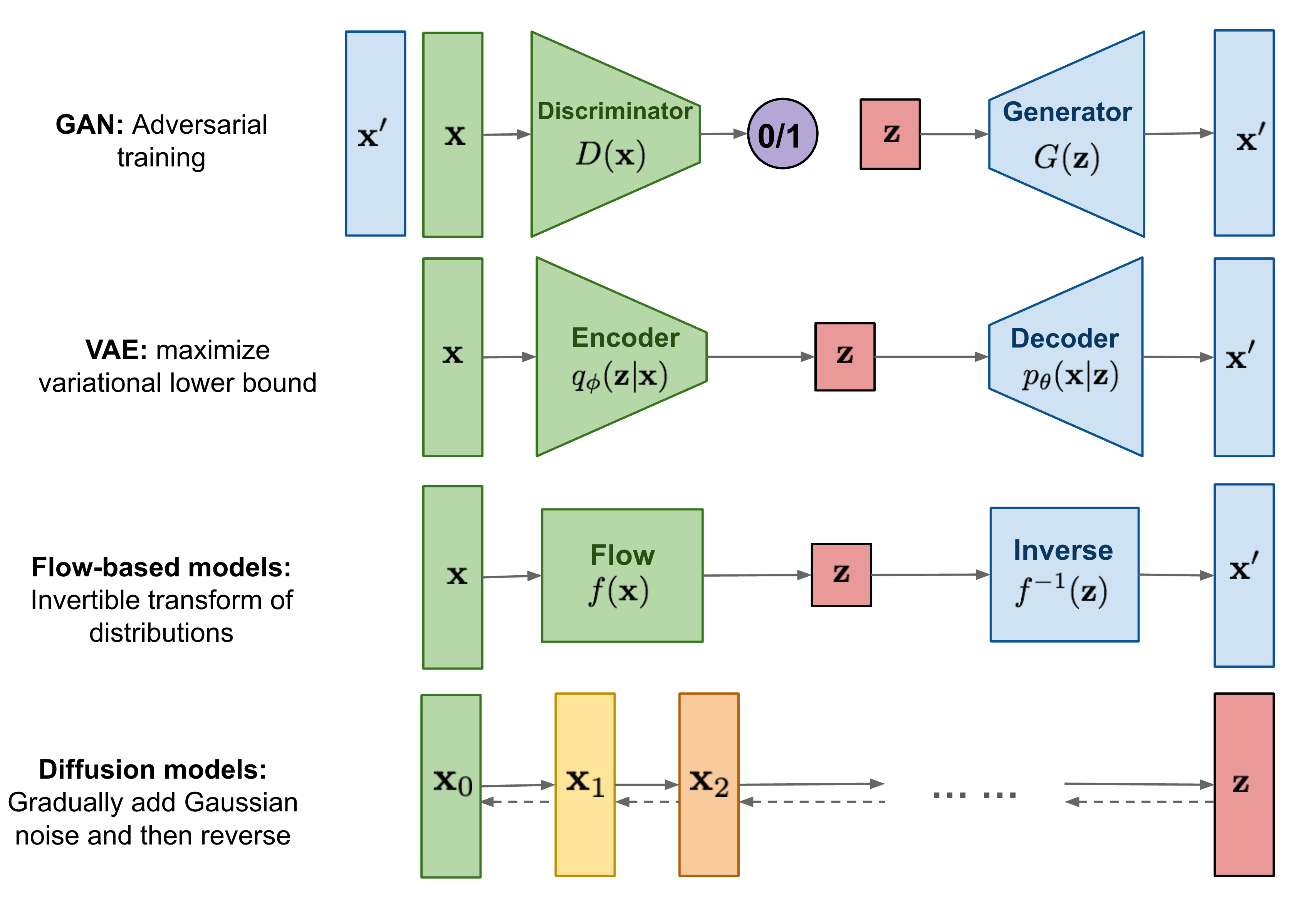
What are Diffusion Models?
Multiple diffusion-based generative modeling approaches have been introduced that share the same underlying principles, including diffusion probabilistic models (Sohl-Dickstein et al., 2015), noise-conditioned score network (NCSN; Yang & Ermon, 2019), and denoising diffusion probabilistic models (DDPM; Ho et al. 2020).
Forward diffusion process
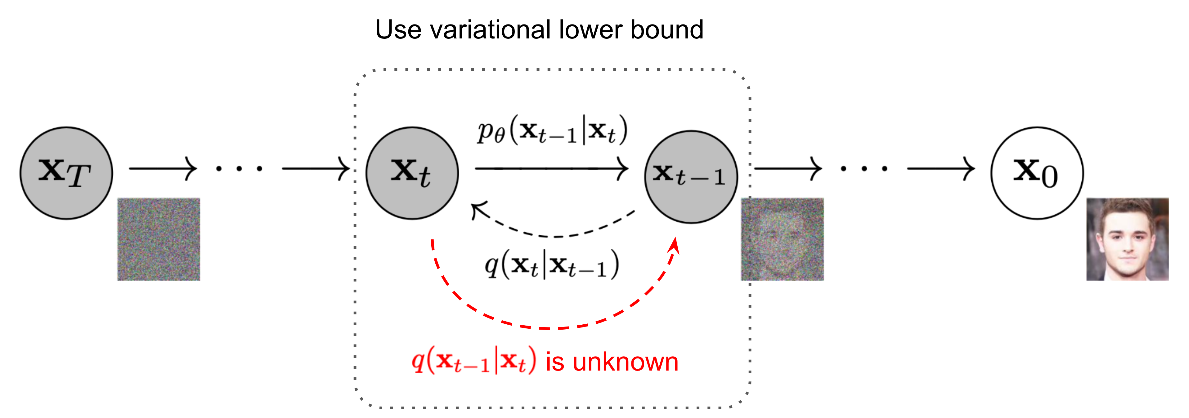
Given a data point sampled from a real data distribution $\mathbf{x}_0 \sim q(\mathbf{x})$, we define a forward diffusion process that adds a small amount of Gaussian noise to the sample over $T$ steps, yielding a sequence of noisy samples $\mathbf{x}_1, \dots, \mathbf{x}_T$. The per-step magnitudes are determined by a variance schedule $\{\beta_t \in (0, 1)\}_{t=1}^T$.
As $t$ increases, the sample $\mathbf{x}_0$ progressively loses distinguishing structure. Ultimately, when $T \to \infty$, $\mathbf{x}_T$ becomes equivalent to an isotropic Gaussian distribution.
An especially convenient property of this process is that we can sample $\mathbf{x}_t$ at any chosen time step $t$ in closed form using the reparameterization trick. Define $\alpha_t = 1 - \beta_t$ and $\bar{\alpha}_t = \prod_{i=1}^t \alpha_i$:
(*) Recall that when we merge two Gaussians with different variances, $\mathcal{N}(\mathbf{0}, \sigma_1^2\mathbf{I})$ and $\mathcal{N}(\mathbf{0}, \sigma_2^2\mathbf{I})$, the resulting distribution is $\mathcal{N}(\mathbf{0}, (\sigma_1^2 + \sigma_2^2)\mathbf{I})$. In this case, the merged standard deviation is $\sqrt{(1 - \alpha_t) + \alpha_t (1-\alpha_{t-1})} = \sqrt{1 - \alpha_t\alpha_{t-1}}$.
In practice, larger update steps are typically affordable as the sample becomes noisier, so $\beta_1 < \beta_2 < \dots < \beta_T$ and therefore $\bar{\alpha}_1 > \dots > \bar{\alpha}_T$.
Connection with stochastic gradient Langevin dynamics
Langevin dynamics is a physics concept developed for statistical modeling of molecular systems. When combined with stochastic gradient descent, stochastic gradient Langevin dynamics (Welling & Teh 2011) can generate samples from a probability density $p(\mathbf{x})$ using only gradients $\nabla_\mathbf{x} \log p(\mathbf{x})$, via the following Markov chain update:
where $\delta$ denotes the step size. When $T \to \infty, \epsilon \to 0$, $\mathbf{x}_T$ equals the true probability density $p(\mathbf{x})$.
Relative to standard SGD, stochastic gradient Langevin dynamics injects Gaussian noise into parameter updates, helping to prevent collapse into local minima.
Reverse diffusion process
If we can invert the process above and sample from $q(\mathbf{x}_{t-1} \vert \mathbf{x}_t)$, then we can reconstruct real samples from Gaussian noise inputs, $\mathbf{x}_T \sim \mathcal{N}(\mathbf{0}, \mathbf{I})$. Observe that if $\beta_t$ is sufficiently small, then $q(\mathbf{x}_{t-1} \vert \mathbf{x}_t)$ will also be Gaussian. Unfortunately, $q(\mathbf{x}_{t-1} \vert \mathbf{x}_t)$ is not easy to estimate because it depends on the entire dataset. Therefore, we train a model $p_\theta$ to approximate these conditional probabilities so we can execute the reverse diffusion process.
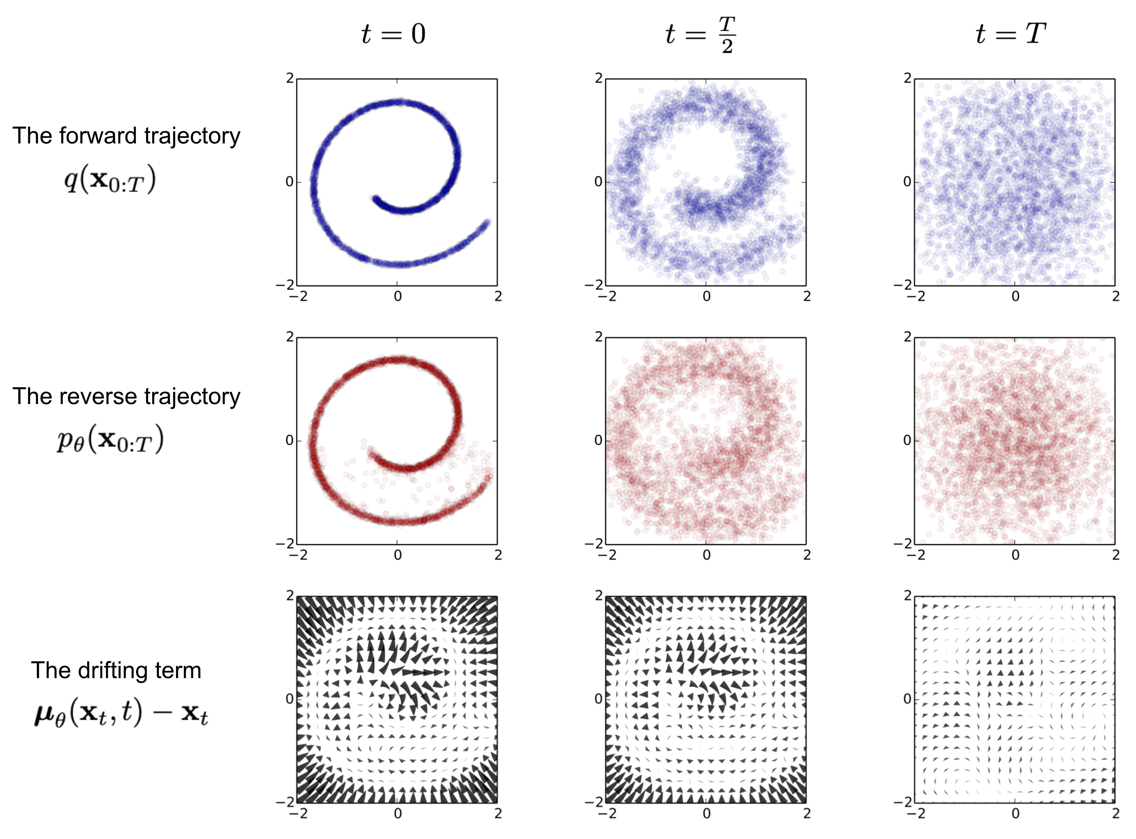
Notably, the reverse conditional probability becomes tractable when conditioned on $\mathbf{x}_0$:
Applying Bayes’ rule yields:
where $C(\mathbf{x}_t, \mathbf{x}_0)$ is a function that does not involve $\mathbf{x}_{t-1}$, and the details are omitted. Using the standard Gaussian density form, we can parameterize the mean and variance as follows (recall that $\alpha_t = 1 - \beta_t$ and $\bar{\alpha}_t = \prod_{i=1}^t \alpha_i$):
Leveraging the nice property, we can express $\mathbf{x}_0 = \frac{1}{\sqrt{\bar{\alpha}_t}}(\mathbf{x}_t - \sqrt{1 - \bar{\alpha}_t}\boldsymbol{\epsilon}_t)$, substitute it into the equation above, and obtain:
As illustrated in Fig. 2., this construction closely mirrors a VAE, and we can therefore optimize the negative log-likelihood through the variational lower bound.
The same conclusion can also be derived directly from Jensen’s inequality. Suppose we minimize cross entropy as the learning objective:
To make every term analytically computable, the objective can be rewritten as a combination of KL-divergence and entropy terms (see the detailed step-by-step derivation in Appendix B of Sohl-Dickstein et al., 2015):
We can label each component of the variational lower bound loss separately:
Each KL term in $L_\text{VLB}$ (except $L_0$) compares two Gaussian distributions, and can therefore be computed in closed form. $L_T$ is constant and can be ignored during training because $q$ contains no learnable parameters and $\mathbf{x}_T$ is Gaussian noise. Ho et al. 2020 models $L_0$ using a separate discrete decoder derived from $\mathcal{N}(\mathbf{x}_0; \boldsymbol{\mu}_\theta(\mathbf{x}_1, 1), \boldsymbol{\Sigma}_\theta(\mathbf{x}_1, 1))$.
Parameterization of $L_t$ for Training Loss
Recall that we train a neural network to approximate the conditional probability distributions in the reverse diffusion process, $p_\theta(\mathbf{x}_{t-1} \vert \mathbf{x}_t) = \mathcal{N}(\mathbf{x}_{t-1}; \boldsymbol{\mu}_\theta(\mathbf{x}_t, t), \boldsymbol{\Sigma}_\theta(\mathbf{x}_t, t))$. The goal is to train $\boldsymbol{\mu}_\theta$ to predict $\tilde{\boldsymbol{\mu}}_t = \frac{1}{\sqrt{\alpha_t}} \Big( \mathbf{x}_t - \frac{1 - \alpha_t}{\sqrt{1 - \bar{\alpha}_t}} \boldsymbol{\epsilon}_t \Big)$. Since $\mathbf{x}_t$ is available as input during training, we can instead reparameterize the Gaussian noise term, training the model to predict $\boldsymbol{\epsilon}_t$ given input $\mathbf{x}_t$ at time step $t$:
The loss term $L_t$ is parameterized to minimize the discrepancy from $\tilde{\boldsymbol{\mu}}$:
Simplification
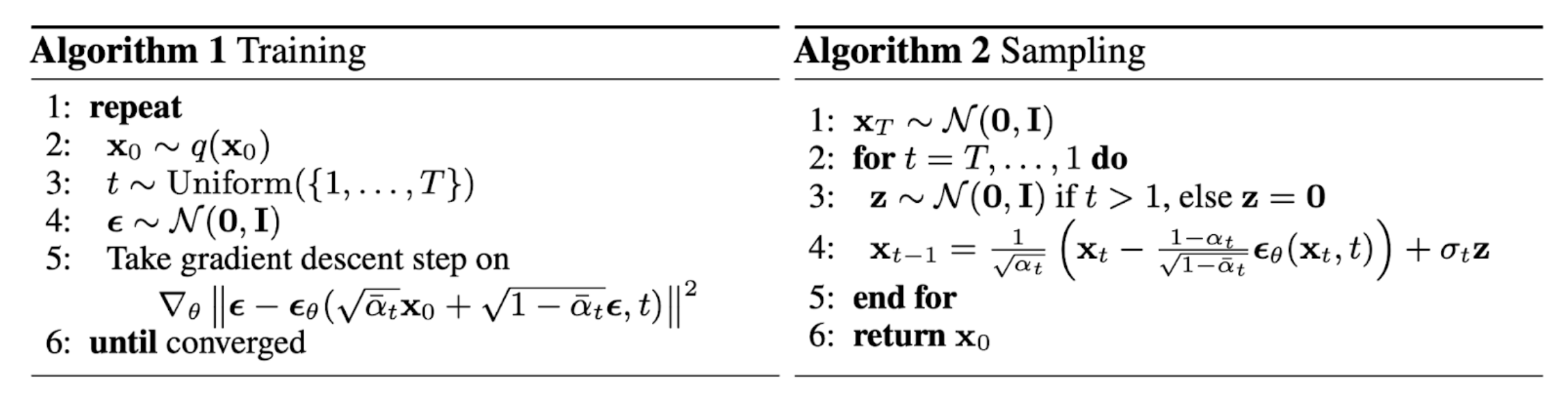
Empirically, Ho et al. (2020) reported that diffusion models train more effectively under a simplified objective that drops the weighting term:
The resulting simplified objective is:
where $C$ is a constant that does not depend on $\theta$.
Connection with noise-conditioned score networks (NCSN)
Song & Ermon (2019) introduced a score-based generative modeling approach in which samples are generated through Langevin dynamics, using gradients of the data distribution estimated via score matching. The score of a sample $\mathbf{x}$’s density is defined as the gradient $\nabla_{\mathbf{x}} \log q(\mathbf{x})$. A score network $\mathbf{s}_\theta: \mathbb{R}^D \to \mathbb{R}^D$ is trained to estimate this quantity, $\mathbf{s}_\theta(\mathbf{x}) \approx \nabla_{\mathbf{x}} \log q(\mathbf{x})$.
To scale to high-dimensional data in deep learning settings, they proposed either denoising score matching (Vincent, 2011) or sliced score matching (using random projections; Song et al., 2019). Denoising score matching adds a pre-specified small noise to the data $q(\tilde{\mathbf{x}} \vert \mathbf{x})$ and estimates $q(\tilde{\mathbf{x}})$ using score matching.
Recall that Langevin dynamics can sample data points from a probability density distribution using only the score $\nabla_{\mathbf{x}} \log q(\mathbf{x})$ through an iterative procedure.
However, under the manifold hypothesis, most data are expected to concentrate on a low-dimensional manifold, even if the observations appear arbitrarily high-dimensional. This concentration can degrade score estimation because samples do not cover the full space. In low-density regions, the estimated score is less trustworthy. By injecting a small Gaussian noise so that the perturbed data distribution covers the full space $\mathbb{R}^D$, training the score estimator becomes more stable. Song & Ermon (2019) further improved this approach by perturbing data with noise at multiple levels, and training a noise-conditioned score network to jointly estimate scores for all perturbed distributions across noise scales.
The increasing noise schedule closely parallels the forward diffusion process. Using diffusion-process notation, the score approximates $\mathbf{s}_\theta(\mathbf{x}_t, t) \approx \nabla_{\mathbf{x}_t} \log q(\mathbf{x}_t)$. For a Gaussian distribution $\mathbf{x} \sim \mathcal{N}(\mathbf{\mu}, \sigma^2 \mathbf{I})$, the derivative of the log density can be written as $\nabla_{\mathbf{x}}\log p(\mathbf{x}) = \nabla_{\mathbf{x}} \Big(-\frac{1}{2\sigma^2}(\mathbf{x} - \boldsymbol{\mu})^2 \Big) = - \frac{\mathbf{x} - \boldsymbol{\mu}}{\sigma^2} = - \frac{\boldsymbol{\epsilon}}{\sigma}$ where $\boldsymbol{\epsilon} \sim \mathcal{N}(\boldsymbol{0}, \mathbf{I})$. Recall that $q(\mathbf{x}_t \vert \mathbf{x}_0) \sim \mathcal{N}(\sqrt{\bar{\alpha}_t} \mathbf{x}_0, (1 - \bar{\alpha}_t)\mathbf{I})$, and therefore:
Parameterization of $\beta_t$
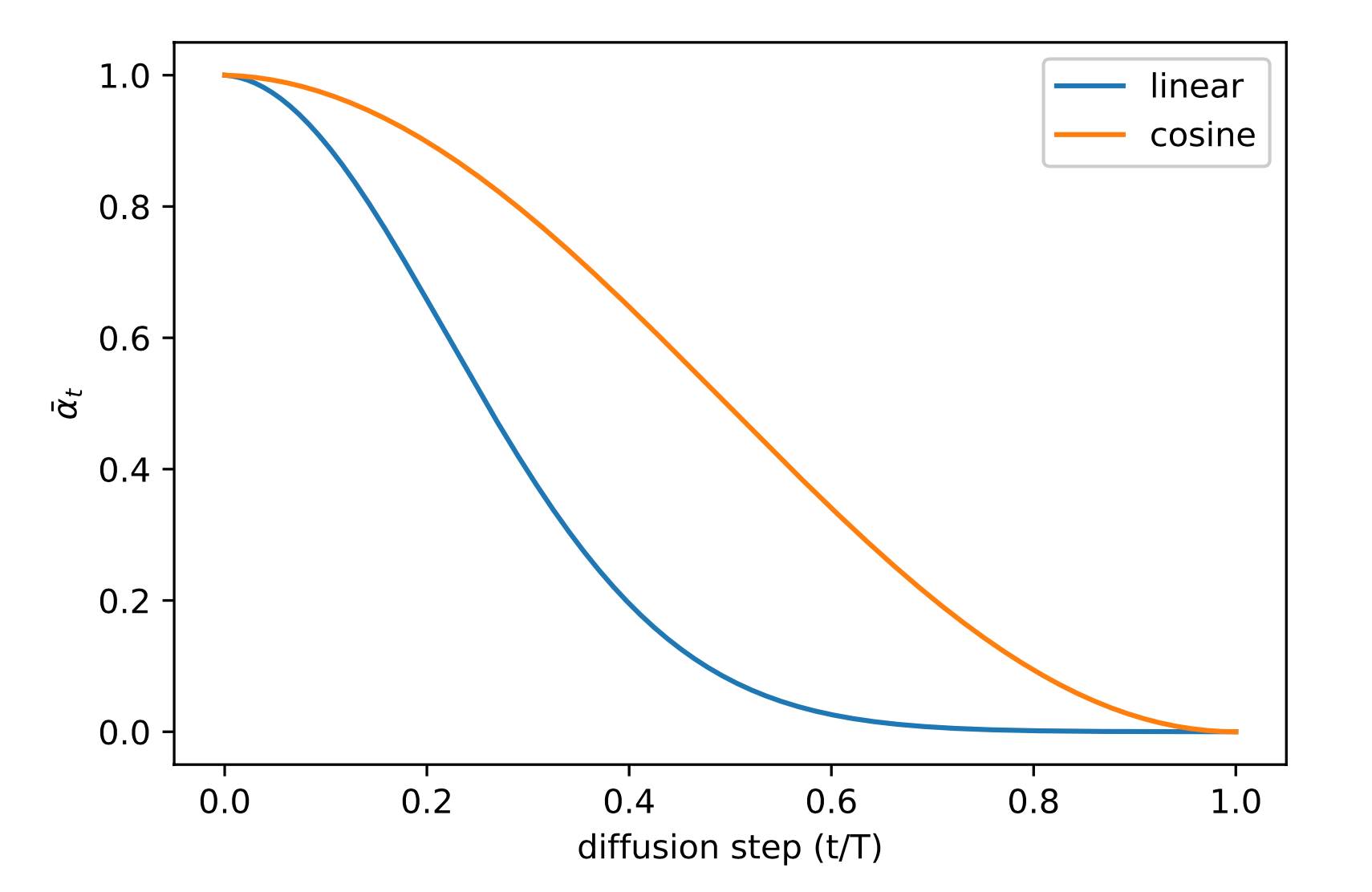
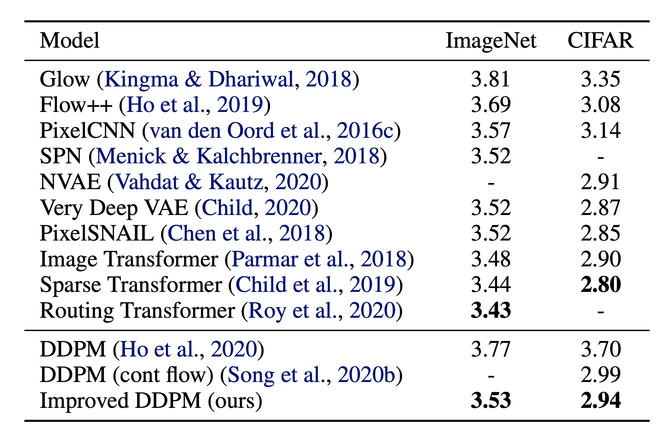
In Ho et al. (2020), the forward variances are set as a linearly increasing sequence of constants, ranging from $\beta_1=10^{-4}$ to $\beta_T=0.02$. These values are small relative to normalized image pixel intensities in the interval $[-1, 1]$. In their experiments, diffusion models produced high-quality samples, but still did not reach model log-likelihood competitiveness with other generative model families.
Nichol & Dhariwal (2021) proposed several improvements aimed at reducing NLL for diffusion models. One improvement is a cosine-based variance schedule. The specific scheduling function may be chosen arbitrarily, provided that it yields a near-linear drop in the middle of training and only mild changes near $t=0$ and $t=T$.
where the small offset $s$ prevents $\beta_t$ from becoming too small when close to $t=0$.
Parameterization of reverse process variance $\boldsymbol{\Sigma}_\theta$
Ho et al. (2020) opted to keep $\beta_t$ fixed as constants rather than making them learnable, and set $\boldsymbol{\Sigma}_\theta(\mathbf{x}_t, t) = \sigma^2_t \mathbf{I}$, where $\sigma_t$ is not learned but instead set to $\beta_t$ or $\tilde{\beta}_t = \frac{1 - \bar{\alpha}_{t-1}}{1 - \bar{\alpha}_t} \cdot \beta_t$. This choice was motivated by their finding that learning a diagonal variance $\boldsymbol{\Sigma}_\theta$ can make training unstable and can degrade sample quality.
Nichol & Dhariwal (2021) proposed learning $\boldsymbol{\Sigma}_\theta(\mathbf{x}_t, t)$ by interpolating between $\beta_t$ and $\tilde{\beta}_t$. In their approach, the model predicts a mixing vector $\mathbf{v}$:
However, the basic objective $L_\text{simple}$ has no dependence on $\boldsymbol{\Sigma}_\theta$. To introduce that dependency, they constructed a hybrid objective $L_\text{hybrid} = L_\text{simple} + \lambda L_\text{VLB}$, where $\lambda=0.001$ is small. They also stop the gradient on $\boldsymbol{\mu}_\theta$ in the $L_\text{VLB}$ term so that $L_\text{VLB}$ provides guidance only for learning $\boldsymbol{\Sigma}_\theta$. Empirically, they observed that $L_\text{VLB}$ is difficult to optimize, likely because the gradients are noisy, so they proposed using a time-averaged, smoothed version of $L_\text{VLB}$ with importance sampling.
Conditioned Generation
When training generative models on images paired with conditioning information (for example, the ImageNet dataset), it is standard to generate samples conditioned on class labels or on a short descriptive text.
Classifier Guided Diffusion
To explicitly incorporate class information into the diffusion process, Dhariwal & Nichol (2021) trained a classifier $f_\phi(y \vert \mathbf{x}_t, t)$ on noisy images $\mathbf{x}_t$ and used gradients $\nabla_\mathbf{x} \log f_\phi(y \vert \mathbf{x}_t)$ to steer the diffusion sampling procedure toward conditioning information $y$ (for example, a target class label) by modifying the noise prediction. Recall that $\nabla_{\mathbf{x}_t} \log q(\mathbf{x}_t) = - \frac{1}{\sqrt{1 - \bar{\alpha}_t}} \boldsymbol{\epsilon}_\theta(\mathbf{x}_t, t)$, and that we can write the score function for the joint distribution $q(\mathbf{x}_t, y)$ as follows:
Accordingly, a classifier-guided predictor $\bar{\boldsymbol{\epsilon}}_\theta$ takes the following form:
To adjust the strength of classifier guidance, we can introduce a weight $w$ on the delta component:
The resulting ablated diffusion model (ADM), as well as the variant with additional classifier guidance (ADM-G), can outperform SOTA generative models (for example, BigGAN).
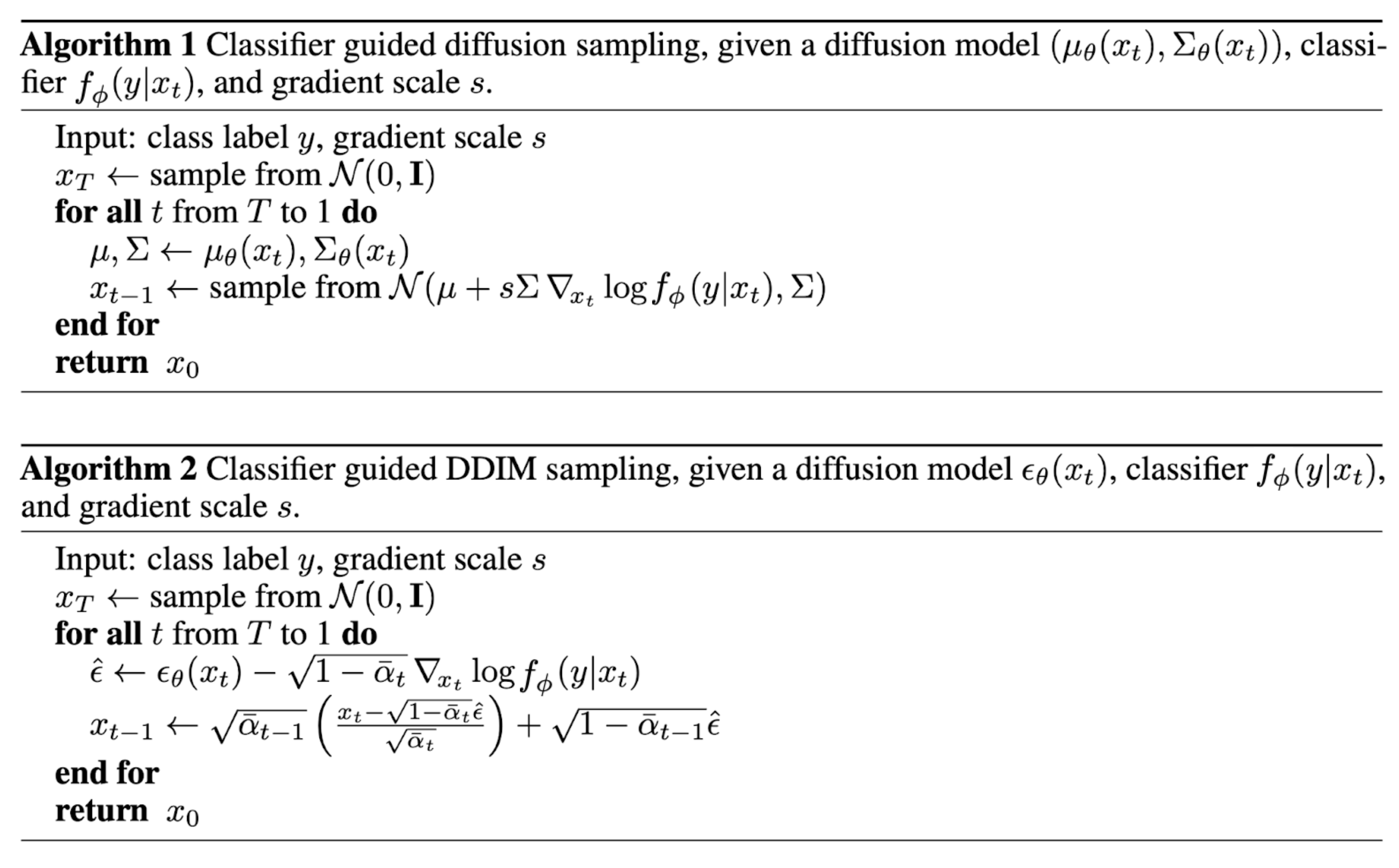
In addition, with several modifications to the U-Net architecture, Dhariwal & Nichol (2021) demonstrated diffusion-model performance that surpasses GANs. Their architectural changes include greater model depth and width, more attention heads, multi-resolution attention, BigGAN residual blocks for upsampling and downsampling, residual-connection rescaling by $1/\sqrt{2}$, and adaptive group normalization (AdaGN).
Classifier-Free Guidance
Even without a separate classifier $f_\phi$, conditional diffusion sampling remains possible by combining the scores from a conditional diffusion model and an unconditional diffusion model (Ho & Salimans, 2021). Let the unconditional denoising diffusion model $p_\theta(\mathbf{x})$ be parameterized by a score estimator $\boldsymbol{\epsilon}_\theta(\mathbf{x}_t, t)$, and let the conditional model $p_\theta(\mathbf{x} \vert y)$ be parameterized by $\boldsymbol{\epsilon}_\theta(\mathbf{x}_t, t, y)$. In practice, both behaviors can be implemented within a single neural network. Specifically, a conditional diffusion model $p_\theta(\mathbf{x} \vert y)$ is trained on paired data $(\mathbf{x}, y)$, where the conditioning information $y$ is randomly dropped at intervals so that the model also learns unconditional generation, that is, $\boldsymbol{\epsilon}_\theta(\mathbf{x}_t, t) = \boldsymbol{\epsilon}_\theta(\mathbf{x}_t, t, y=\varnothing)$.
The gradient of an implicit classifier can be expressed using conditional and unconditional score estimators. When substituted into the classifier-guided modified score, the resulting score no longer depends on a separate classifier.
In their experiments, classifier-free guidance achieved a favorable tradeoff between FID (distinguishing between synthetic and generated images) and IS (quality and diversity).
It is straightforward to see that applying classifier guidance with weight $w$ to a conditional model is equivalent to applying weight $w+1$ to an unconditional model, because:
Therefore, the classifier-guided noise prediction can be rewritten as:
The guided diffusion model, GLIDE (Nichol, Dhariwal & Ramesh, et al. 2022), investigated both guidance strategies (CLIP guidance and classifier-free guidance) and concluded that classifier-free guidance is preferable. They hypothesized that CLIP guidance pushes the model toward adversarial examples for the CLIP model, rather than optimizing generation of better-matched images.
Speed up Diffusion Models
Sampling from a DDPM is slow because it follows the reverse diffusion Markov chain, and $T$ may require one to several thousand steps. As one data point from Song et al. (2020) notes: “For example, it takes around 20 hours to sample 50k images of size 32 × 32 from a DDPM, but less than a minute to do so from a GAN on an Nvidia 2080 Ti GPU.”
Fewer Sampling Steps & Distillation
One straightforward strategy is to use a strided sampling schedule (Nichol & Dhariwal, 2021), taking a sampling update every $\lceil T/S \rceil$ steps and thereby reducing the process from $T$ to $S$ steps. The resulting generation schedule is $\{\tau_1, \dots, \tau_S\}$, where $\tau_1 < \tau_2 < \dots <\tau_S \in [1, T]$ and $S < T$.
As another approach, we can rewrite $q_\sigma(\mathbf{x}_{t-1} \vert \mathbf{x}_t, \mathbf{x}_0)$ so that it is parameterized by a desired standard deviation $\sigma_t$, using the nice property:
where the model $\epsilon^{(t)}_\theta(.)$ predicts $\epsilon_t$ from $\mathbf{x}_t$.
Recall that in $q(\mathbf{x}_{t-1} \vert \mathbf{x}_t, \mathbf{x}_0) = \mathcal{N}(\mathbf{x}_{t-1}; \tilde{\boldsymbol{\mu}}(\mathbf{x}_t, \mathbf{x}_0), \tilde{\beta}_t \mathbf{I})$; therefore, we have:
Let $\sigma_t^2 = \eta \cdot \tilde{\beta}_t$ so that we can treat $\eta \in \mathbb{R}^+$ as a hyperparameter to control sampling stochasticity. In the special case $\eta = 0$, sampling becomes deterministic. This model is called the denoising diffusion implicit model (DDIM; Song et al., 2020). DDIM preserves the same marginal noise distribution while deterministically mapping noise back to the original data samples.
At generation time, it is not necessary to follow the full chain $t=1,\dots,T$; instead, we can sample using only a subset of steps. Let $s < t$ denote two steps along this accelerated trajectory. The DDIM update is:
Although all models in the experiments were trained with $T=1000$ diffusion steps, the authors observed that DDIM ($\eta=0$) can produce the highest-quality samples when $S$ is small, whereas DDPM ($\eta=1$) performs substantially worse for small $S$. DDPM does perform better when the full reverse Markov diffusion process is affordable ($S=T=1000$). With DDIM, it is possible to train a diffusion model with any arbitrary number of forward steps while sampling from only a subset of steps at generation time.
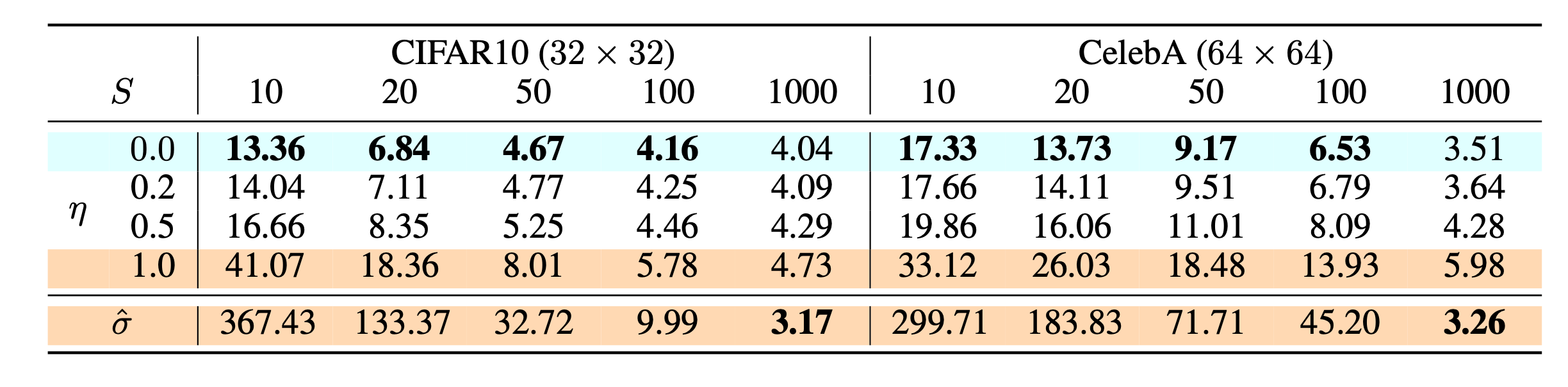
Relative to DDPM, DDIM can:
- Generate higher-quality samples using a much smaller number of steps.
- Exhibit a “consistency” property because the generative process is deterministic, meaning multiple samples conditioned on the same latent variable should share similar high-level features.
- Perform semantically meaningful interpolation in the latent variable because of this consistency.
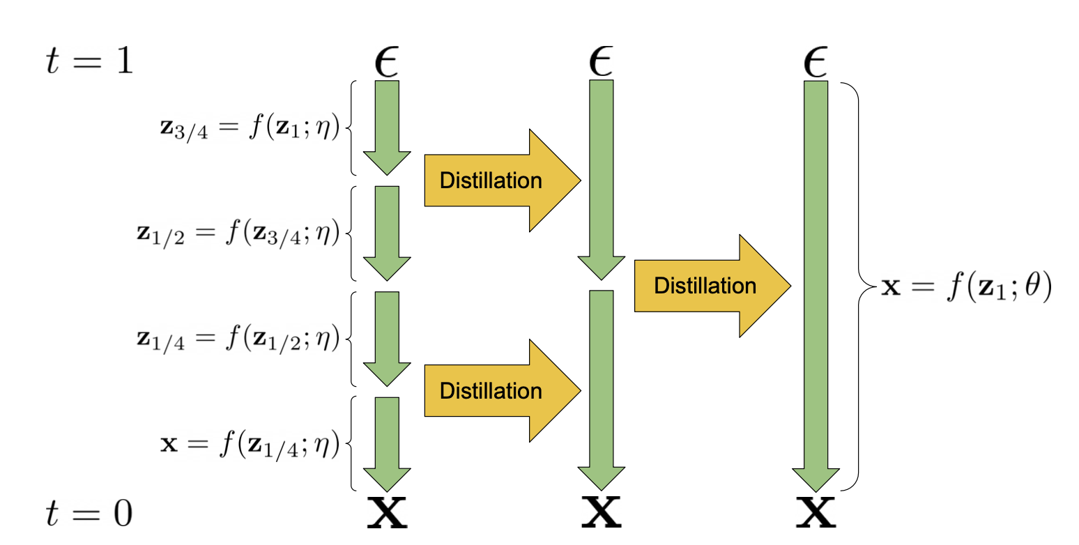
Progressive Distillation (Salimans & Ho, 2022) distills trained deterministic samplers into new models that require half as many sampling steps. The student model is initialized from the teacher model and is trained to denoise toward a target where one student DDIM step matches two teacher steps, rather than using the original sample $\mathbf{x}_0$ as the denoising target. With each progressive distillation iteration, the number of sampling steps can be halved.
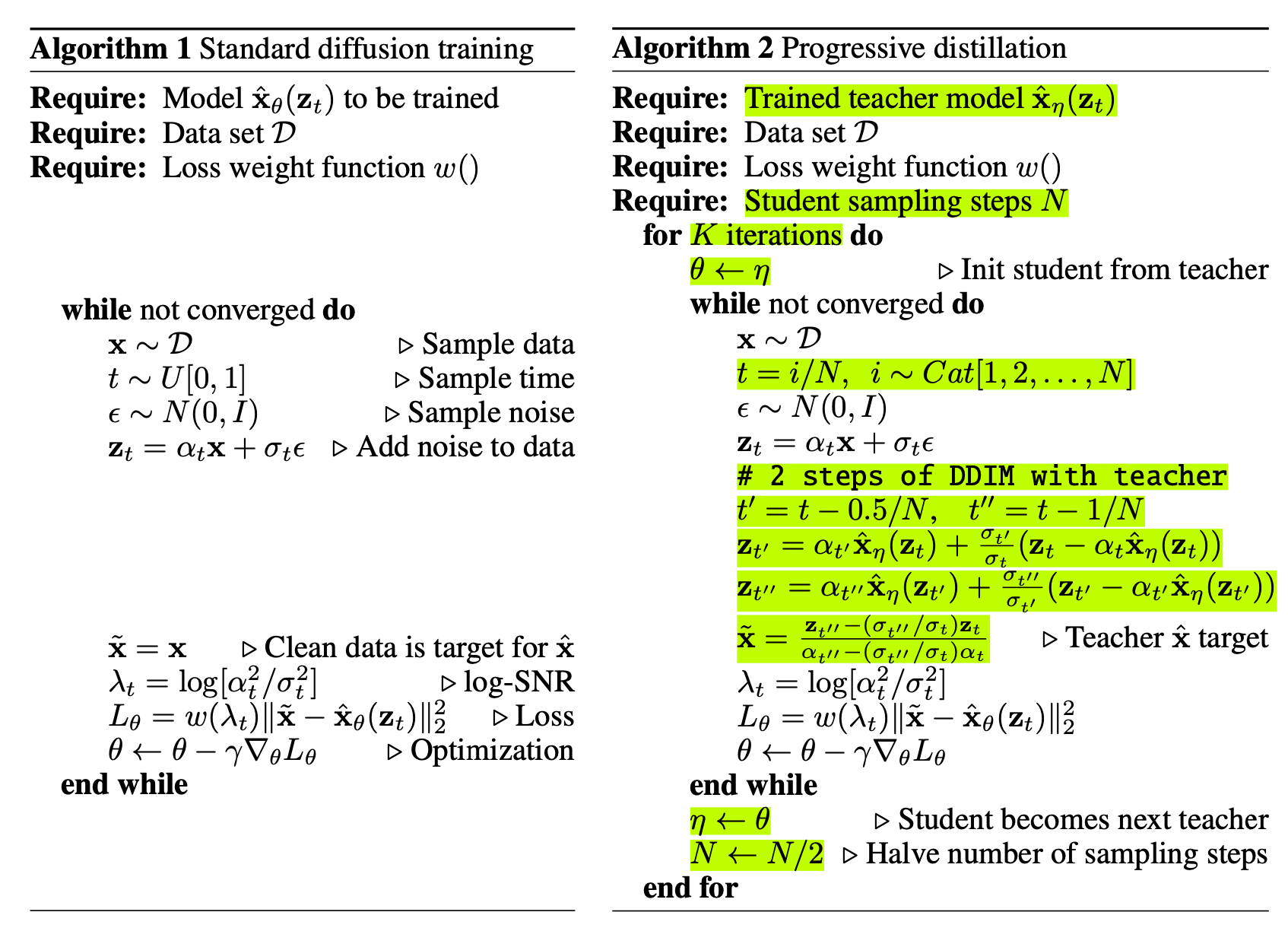
(Image source: Salimans & Ho, 2022)
Consistency Models (Song et al. 2023) learn to map any intermediate noisy data points $\mathbf{x}_t, t > 0$ along a diffusion sampling trajectory directly back to their origin $\mathbf{x}_0$. They are called consistency models because of a self-consistency property: any points along the same trajectory are mapped to the same origin.
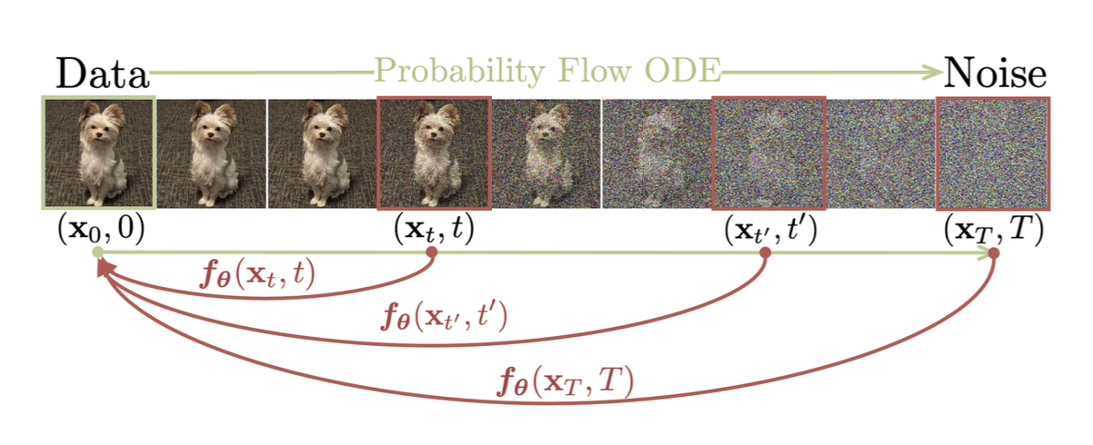
Given a trajectory $\{\mathbf{x}_t \vert t \in [\epsilon, T]\}$, the consistency function $f$ is defined as $f: (\mathbf{x}_t, t) \mapsto \mathbf{x}_\epsilon$, and the equation $f(\mathbf{x}_t, t) = f(\mathbf{x}_{t’}, t’) = \mathbf{x}_\epsilon$ holds for all $t, t’ \in [\epsilon, T]$. When $t=\epsilon$, $f$ is an identify function. The model can be parameterized as follows, where the $c_\text{skip}(t)$ and $c_\text{out}(t)$ functions are constructed so that $c_\text{skip}(\epsilon) = 1, c_\text{out}(\epsilon) = 0$:
A consistency model can generate samples in a single step, while still retaining the option to trade additional computation for higher quality through multi-step sampling.
The paper described two training approaches for consistency models:
-
Consistency Distillation (CD): Distill a diffusion model into a consistency model by minimizing the discrepancy between model outputs for pairs produced from the same trajectory. This enables significantly cheaper sampling evaluation. The consistency distillation loss is:
$ \begin{aligned} \mathcal{L}^N_\text{CD} (\theta, \theta^-; \phi) &= \mathbb{E} [\lambda(t_n)d(f_\theta(\mathbf{x}_{t_{n+1}}, t_{n+1}), f_{\theta^-}(\hat{\mathbf{x}}^\phi_{t_n}, t_n)] \\ \hat{\mathbf{x}}^\phi_{t_n} &= \mathbf{x}_{t_{n+1}} - (t_n - t_{n+1}) \Phi(\mathbf{x}_{t_{n+1}}, t_{n+1}; \phi) \end{aligned} $where:
- $\Phi(.;\phi)$ is the update function of a one-step ODE solver;
- $n \sim \mathcal{U}[1, N-1]$ has an uniform distribution over $1, \dots, N-1$;
- The network parameters $\theta^-$ are the EMA version of $\theta$, which substantially stabilizes training (as in DQN or momentum contrastive learning);
- $d(.,.)$ is a positive distance metric function that satisfies $\forall \mathbf{x}, \mathbf{y}: d(\mathbf{x}, \mathbf{y}) \geq 0$ and $d(\mathbf{x}, \mathbf{y}) = 0$ if and only if $\mathbf{x} = \mathbf{y}$, such as $\ell_2$, $\ell_1$, or LPIPS (learned perceptual image patch similarity) distance;
- $\lambda(.) \in \mathbb{R}^+$ is a positive weighting function, and the paper sets $\lambda(t_n)=1$.
-
Consistency Training (CT): Alternatively, a consistency model can be trained independently. Note that in CD, a pre-trained score model $s_\phi(\mathbf{x}, t)$ is used to approximate the ground-truth score $\nabla\log p_t(\mathbf{x})$, whereas in CT we require a way to estimate this score function. It turns out that an unbiased estimator of $\nabla\log p_t(\mathbf{x})$ exists as $-\frac{\mathbf{x}_t - \mathbf{x}}{t^2}$. The CT loss is defined as follows:
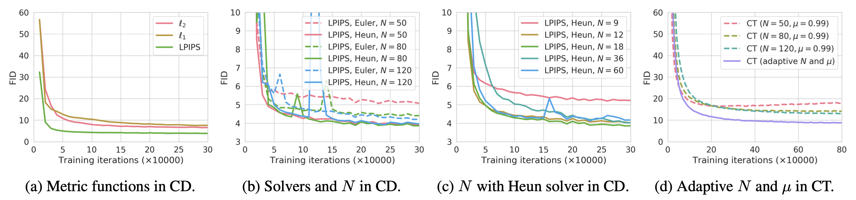
Based on the experiments reported in the paper, the authors found:
- The Heun ODE solver performs better than Euler’s first-order solver, because higher-order ODE solvers have smaller estimation errors for the same $N$.
- Across choices of the distance metric function $d(.)$, the LPIPS metric outperforms $\ell_1$ and $\ell_2$ distance.
- Smaller $N$ yields faster convergence but lower-quality samples, whereas larger $N$ yields slower convergence but better samples at convergence.
Latent Variable Space
Latent diffusion model (LDM; Rombach & Blattmann, et al. 2022) runs diffusion in latent space rather than pixel space, reducing training cost and accelerating inference. This is motivated by the observation that most bits in an image contribute to perceptual detail, while semantic and conceptual structure can persist even after aggressive compression. LDM loosely separates perceptual compression from semantic compression in generative modeling: it first removes pixel-level redundancy using an autoencoder, then manipulates or generates semantic concepts by running the diffusion process on the learned latent representation.
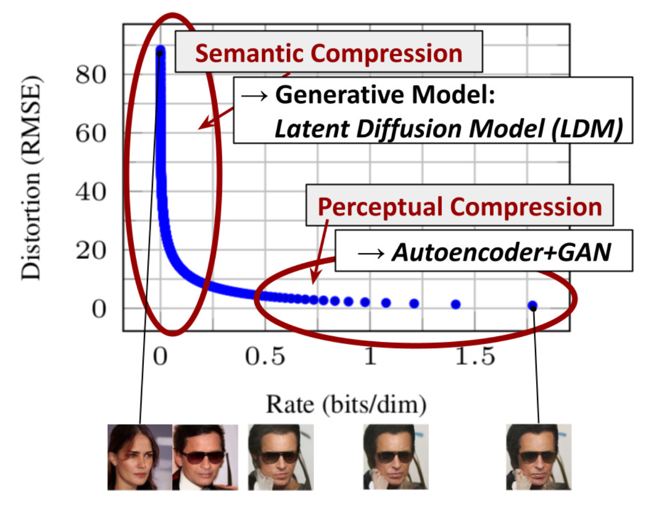
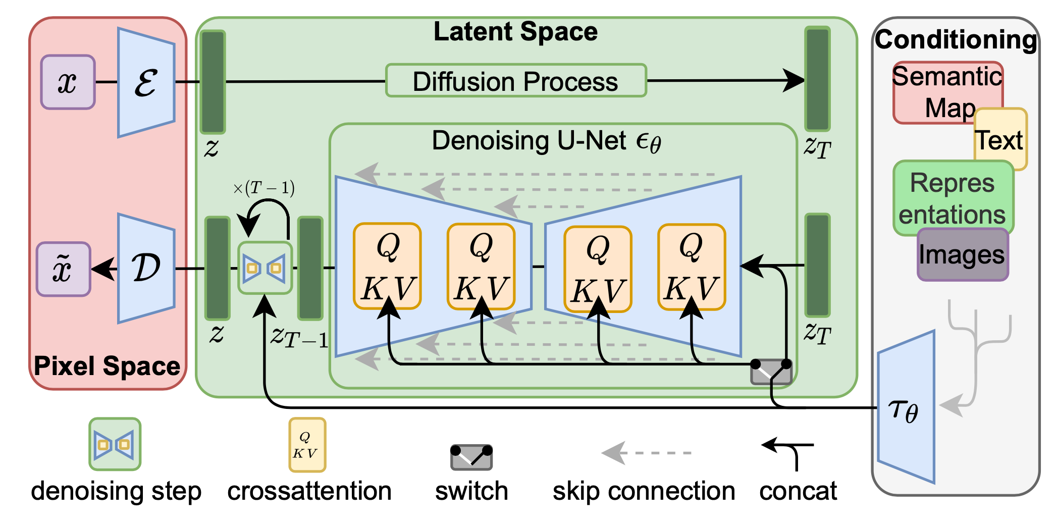
Perceptual compression relies on an autoencoder. An encoder $\mathcal{E}$ compresses the input image $\mathbf{x} \in \mathbb{R}^{H \times W \times 3}$ into a smaller 2D latent vector $\mathbf{z} = \mathcal{E}(\mathbf{x}) \in \mathbb{R}^{h \times w \times c}$, with downsampling rate $f=H/h=W/w=2^m, m \in \mathbb{N}$. A decoder $\mathcal{D}$ then reconstructs images from the latent vector, $\tilde{\mathbf{x}} = \mathcal{D}(\mathbf{z})$. The paper explored two regularization approaches for autoencoder training to prevent arbitrarily high variance in latent space.
- KL-reg: Adds a small KL penalty toward a standard normal distribution over the learned latent, similar to VAE.
- VQ-reg: Introduces a vector-quantization layer within the decoder, as in VQVAE, but the quantization layer is absorbed by the decoder.
Diffusion and denoising are performed on the latent vector $\mathbf{z}$. The denoising model is a time-conditioned U-Net augmented with cross-attention to support flexible conditioning inputs for image generation (for example, class labels, semantic maps, and blurred variants of an image). Conceptually, this design fuses representations from different modalities via cross-attention. Each conditioning type is paired with a domain-specific encoder $\tau_\theta$ that projects the conditioning input $y$ into an intermediate representation that can be mapped into the cross-attention component, $\tau_\theta(y) \in \mathbb{R}^{M \times d_\tau}$:
Scale up Generation Resolution and Quality
To generate high-quality images at high resolution, Ho et al. (2021) proposed a pipeline of multiple diffusion models operating at progressively higher resolutions. Noise conditioning augmentation between pipeline stages is critical to final image quality. The idea is to apply strong data augmentation to the conditioning input $\mathbf{z}$ for each super-resolution model $p_\theta(\mathbf{x} \vert \mathbf{z})$. This conditioning noise reduces compounding errors in the pipeline. U-net is a common architectural choice in diffusion modeling for high-resolution image generation.
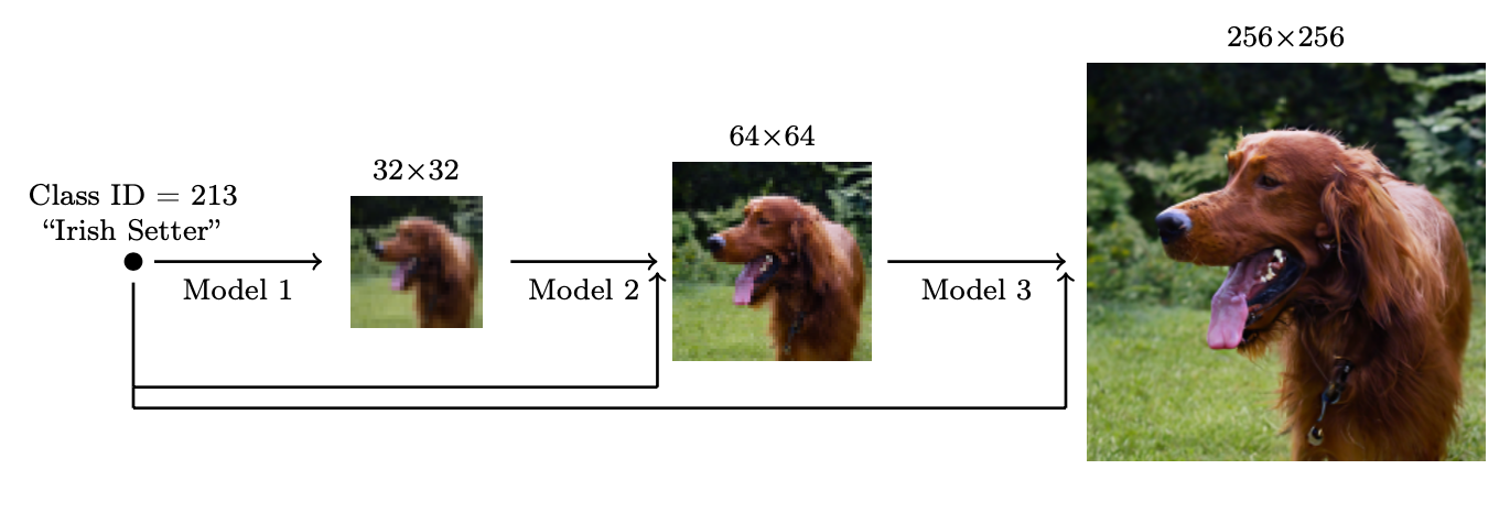
They found that the most effective noise strategy is to apply Gaussian noise at low resolution and Gaussian blur at high resolution. They also explored two additional forms of conditioning augmentation that require only small changes to the training procedure. Note that conditioning noise is applied during training only, not during inference.
- Truncated conditioning augmentation stops the diffusion process early at step $t > 0$ for low resolution.
- Non-truncated conditioning augmentation runs the full low-resolution reverse process through step 0, then corrupts it by $\mathbf{z}_t \sim q(\mathbf{x}_t \vert \mathbf{x}_0)$ and feeds the corrupted $\mathbf{z}_t$ s into the super-resolution model.
The two-stage diffusion model unCLIP (Ramesh et al. 2022) makes extensive use of the CLIP text encoder to generate high-quality, text-guided images. Given a pretrained CLIP model $\mathbf{c}$ and paired diffusion-model training data $(\mathbf{x}, y)$, where $x$ is an image and $y$ is the corresponding caption, we can compute the CLIP text and image embeddings, $\mathbf{c}^t(y)$ and $\mathbf{c}^i(\mathbf{x})$, respectively. unCLIP learns two models in parallel:
- A prior model $P(\mathbf{c}^i \vert y)$: outputs the CLIP image embedding $\mathbf{c}^i$ given the text $y$.
- A decoder $P(\mathbf{x} \vert \mathbf{c}^i, [y])$: generates the image $\mathbf{x}$ given the CLIP image embedding $\mathbf{c}^i$ and, optionally, the original text $y$.
These two models support conditional generation because
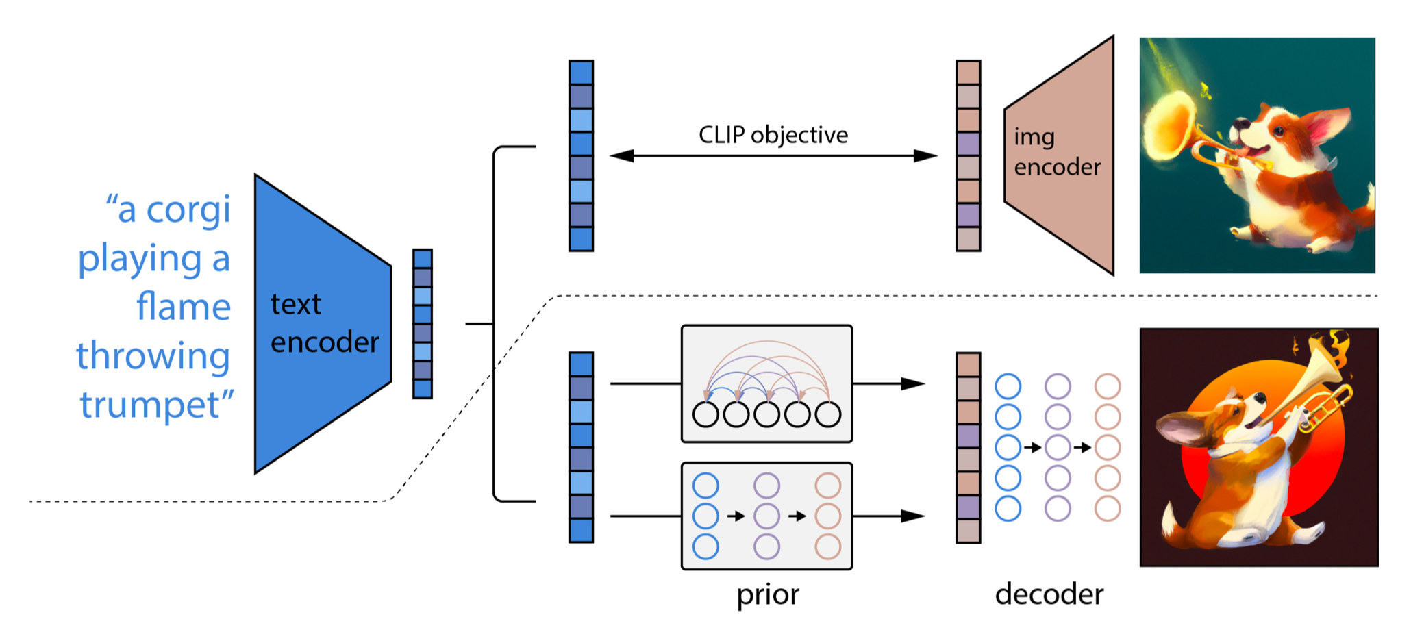
unCLIP uses a two-stage image generation pipeline:
- Given a text $y$, a CLIP model is used first to produce a text embedding $\mathbf{c}^t(y)$. Operating in the CLIP latent space enables zero-shot image manipulation driven by text.
- A diffusion or autoregressive prior $P(\mathbf{c}^i \vert y)$ takes this CLIP text embedding, constructs an image prior, and then a diffusion decoder $P(\mathbf{x} \vert \mathbf{c}^i, [y])$ generates an image conditioned on that prior. This decoder can also create image variations conditioned on an input image, while preserving the input’s style and semantics.
Rather than using a CLIP model, Imagen (Saharia et al. 2022) relies on a pre-trained large language model (that is, a frozen T5-XXL text encoder) to encode text for image generation. A broad trend is that increasing model size can improve both image quality and text-image alignment. The authors report that T5-XXL and the CLIP text encoder perform similarly on MS-COCO, while human evaluators prefer T5-XXL on DrawBench (a prompt collection spanning 11 categories).
With classifier-free guidance, increasing $w$ can improve image-text alignment but degrade image fidelity. The authors attribute this to a train-test mismatch: because the training data $\mathbf{x}$ remains within the range $[-1, 1]$, the test-time data should remain within that range as well. They propose two thresholding strategies:
- Static thresholding: clip the $\mathbf{x}$ prediction to $[-1, 1]$.
- Dynamic thresholding: at each sampling step, compute $s$ as a chosen percentile of the absolute pixel values; if $s > 1$, clip the prediction to $[-s, s]$ and divide by $s$.
Imagen also adjusts several U-Net design choices to create an efficient U-Net.
- Shift model parameters from high-resolution blocks to low-resolution blocks by adding more residual locks for lower resolutions.
- Scale the skip connections by $1/\sqrt{2}$.
- Reverse the order of downsampling (move it before convolutions) and upsampling operations (move it after convolution) to improve forward-pass speed.
They found that noise conditioning augmentation, dynamic thresholding, and efficient U-Net are critical to image quality, while scaling the text encoder size matters more than scaling the U-Net size.
Model Architecture
Two backbone architecture families are commonly used for diffusion models: U-Net and Transformer.
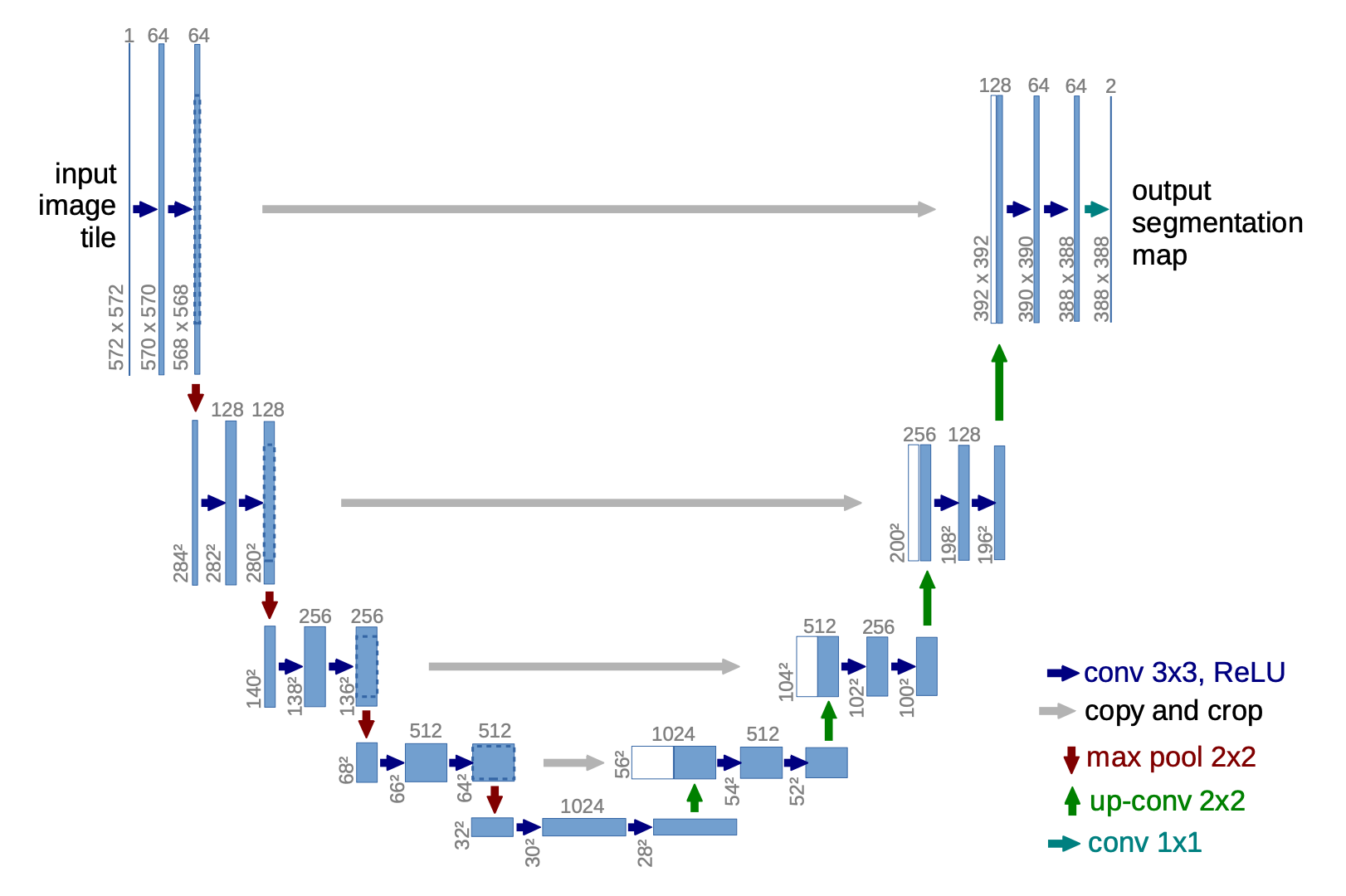
U-Net (Ronneberger, et al. 2015) is composed of a downsampling stack and an upsampling stack.
- Downsampling: Each step applies two 3x3 convolutions (unpadded convolutions), each followed by a ReLU, and then a 2x2 max pooling with stride 2. At each downsampling step, the number of feature channels is doubled.
- Upsampling: Each step upsamples the feature map and then applies a 2x2 convolution; each step halves the number of feature channels.
- Shortcuts: Shortcut connections concatenate features with the corresponding layers in the downsampling stack, supplying the high-resolution information required by the upsampling process.
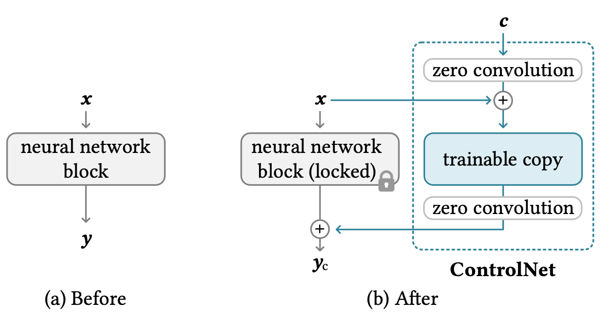
To support image generation conditioned on additional images that convey composition information (for example, Canny edges, Hough lines, user scribbles, human post skeletons, segmentation maps, depths, and normals), ControlNet (Zhang et al. 2023 introduces architectural modifications by inserting “sandwiched” zero convolution layers and a trainable copy of the original model weights into each encoder layer of the U-Net. Concretely, given a neural network block $\mathcal{F}_\theta(.)$, ControlNet proceeds as follows:
- First, freeze the original parameters $\theta$ of the original block.
- Clone the block to create a copy with trainable parameters $\theta_c$ and an additional conditioning vector $\mathbf{c}$.
- Connect the two blocks using two zero convolution layers, denoted $\mathcal{Z}_{\theta_{z1}}(.;.)$ and $\mathcal{Z}_{\theta_{z2}}(.;.)$, which are 1x1 convo layers whose weights and biases are initialized to zeros. Zero convolutions protect this back-bone by eliminating random noise as gradients during the initial training steps.
- The final output is: $\mathbf{y}_c = \mathcal{F}_\theta(\mathbf{x}) + \mathcal{Z}_{\theta_{z2}}(\mathcal{F}_{\theta_c}(\mathbf{x} + \mathcal{Z}_{\theta_{z1}}(\mathbf{c})))$
Diffusion Transformer (DiT; Peebles & Xie, 2023) performs diffusion modeling over latent patches, using the same design space as LDM (Latent Diffusion Model)]. DiT uses the following configuration:
- Use the latent representation of an input $\mathbf{z}$ as the input to DiT.
- “Patchify” the noise latent of size $I \times I \times C$ into patches of size $p$, then convert it into a patch sequence of size $(I/p)^2$.
- Pass this token sequence through Transformer blocks. The authors explore three approaches to conditioning generation on contextual information such as timestep $t$ or class label $c$. Among the three, adaLN (Adaptive layer norm)-Zero performs best, exceeding both in-context conditioning and a cross-attention block. The scale and shift parameters, $\gamma$ and $\beta$, are regressed from the sum of the embedding vectors of $t$ and $c$. The dimension-wise scaling parameters $\alpha$ are also regressed and applied immediately before any residual connections within the DiT block.
- The Transformer decoder produces noise predictions and a diagonal covariance prediction for the output.
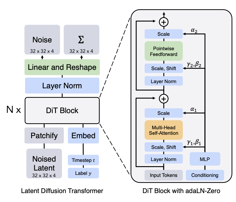
(Image source: Peebles & Xie, 2023)
Transformer architectures are well known for scaling effectively, and they can be expanded straightforwardly. This is a major advantage of DiT: experimental results show that performance improves with additional compute, and that larger DiT models are more compute efficient.
Quick Summary
-
Pros: Tractability and flexibility are competing objectives in generative modeling. Tractable models can be evaluated analytically and fit data inexpensively (for example, via a Gaussian or Laplace), but they cannot easily represent the structure of rich datasets. Flexible models can capture arbitrary structure in data, but evaluation, training, or sampling is typically expensive. Diffusion models are both analytically tractable and flexible.
-
Cons: Diffusion models generate samples through a long Markov chain of diffusion steps, which can be costly in time and compute. Although newer methods can accelerate the process substantially, sampling remains slower than GAN.
Citation
Cited as:
Weng, Lilian. (Jul 2021). What are diffusion models? Lil’Log. https://lilianweng.github.io/posts/2021-07-11-diffusion-models/.
Or
@article{weng2021diffusion,
  title   = "What are diffusion models?",
  author  = "Weng, Lilian",
  journal = "lilianweng.github.io",
  year    = "2021",
  month   = "Jul",
  url     = "https://lilianweng.github.io/posts/2021-07-11-diffusion-models/"
}
References
[1] Jascha Sohl-Dickstein et al. “Deep Unsupervised Learning using Nonequilibrium Thermodynamics.” ICML 2015.
[2] Max Welling & Yee Whye Teh. “Bayesian learning via stochastic gradient langevin dynamics.” ICML 2011.
[3] Yang Song & Stefano Ermon. “Generative modeling by estimating gradients of the data distribution.” NeurIPS 2019.
[4] Yang Song & Stefano Ermon. “Improved techniques for training score-based generative models.” NeuriPS 2020.
[5] Jonathan Ho et al. “Denoising diffusion probabilistic models.” arxiv Preprint arxiv:2006.11239 (2020). [code]
[6] Jiaming Song et al. “Denoising diffusion implicit models.” arxiv Preprint arxiv:2010.02502 (2020). [code]
[7] Alex Nichol & Prafulla Dhariwal. “Improved denoising diffusion probabilistic models” arxiv Preprint arxiv:2102.09672 (2021). [code]
[8] Prafula Dhariwal & Alex Nichol. “Diffusion Models Beat GANs on Image Synthesis.” arxiv Preprint arxiv:2105.05233 (2021). [code]
[9] Jonathan Ho & Tim Salimans. “Classifier-Free Diffusion Guidance.” NeurIPS 2021 Workshop on Deep Generative Models and Downstream Applications.
[10] Yang Song, et al. “Score-Based Generative Modeling through Stochastic Differential Equations.” ICLR 2021.
[11] Alex Nichol, Prafulla Dhariwal & Aditya Ramesh, et al. “GLIDE: Towards Photorealistic Image Generation and Editing with Text-Guided Diffusion Models.” ICML 2022.
[12] Jonathan Ho, et al. “Cascaded diffusion models for high fidelity image generation.” J. Mach. Learn. Res. 23 (2022): 47-1.
[13] Aditya Ramesh et al. “Hierarchical Text-Conditional Image Generation with CLIP Latents.” arxiv Preprint arxiv:2204.06125 (2022).
[14] Chitwan Saharia & William Chan, et al. “Photorealistic Text-to-Image Diffusion Models with Deep Language Understanding.” arxiv Preprint arxiv:2205.11487 (2022).
[15] Rombach & Blattmann, et al. “High-Resolution Image Synthesis with Latent Diffusion Models.” CVPR 2022.code
[16] Song et al. “Consistency Models” arxiv Preprint arxiv:2303.01469 (2023)
[17] Salimans & Ho. “Progressive Distillation for Fast Sampling of Diffusion Models” ICLR 2022.
[18] Ronneberger, et al. “U-Net: Convolutional Networks for Biomedical Image Segmentation” MICCAI 2015.
[19] Peebles & Xie. “Scalable diffusion models with transformers.” ICCV 2023.
[20] Zhang et al. “Adding Conditional Control to Text-to-Image Diffusion Models.” arxiv Preprint arxiv:2302.05543 (2023).