Large Transformer Model Inference Optimization
[Updated on 2023-01-24: add a small section on Distillation.] Large transformer models are now widely used, delivering state-of-the-art (SoTA) results across a broad range of tasks. However, they are both costly to train and expensive to operate. The very high inference cost, in terms of both latency and memory footprint, remains a major bottleneck to deploying powerful transformers for real-world, large-scale workloads. Why is inference for large transformer models so difficult, In addition to the growing size of SoTA models, two primary factors contribute to the inference challenge (Pope et al. 2022):
· 9 min read · Curated and presented by Arthur Sedek
[Updated on 2023-01-24: add a small section on Distillation.]
Large transformer models are now widely used and routinely achieve state-of-the-art (SoTA) results across many tasks. However, they are costly to train and to serve. In particular, the very high cost of inference, in both runtime and memory consumption, is a major barrier to deploying large transformers for real-world, large-scale applications.
Why is it difficult to run inference for large transformer models? In addition to the steady growth in SoTA model sizes, two primary factors drive the inference challenge (Pope et al. 2022):
- Large memory footprint. Inference requires keeping both model parameters and intermediate states resident in memory. For example,
- The KV cache must be stored in memory during decoding; e.g., with a batch size of 512 and a context length of 2048, the KV cache totals 3TB, which is 3x the model size (!).
- The attention mechanism incurs inference costs that scale quadratically with the input sequence length.
- Low parallelizability. Output generation is autoregressive, which makes the decoding procedure inherently difficult to parallelize.
This post examines multiple approaches for improving transformer inference efficiency. Some are general-purpose network compression techniques, while others target the transformer architecture specifically.
Methods Overview
In general, we treat the following as key objectives for inference optimization:
- Reduce the model’s memory footprint so that it can run on fewer GPU devices and consume less GPU memory.
- Reduce computational demands by lowering the number of required FLOPs.
- Reduce end-to-end inference latency and increase throughput.
A number of techniques can reduce inference cost in memory and/or time:
- Apply different forms of parallelism to distribute the model across many GPUs. With well-designed parallelization of model components and data, it becomes feasible to serve models with trillions of parameters.
- Use memory offloading by moving temporarily unused data to CPU memory and retrieving it later when needed. This reduces GPU memory usage, but typically increases latency.
- Adopt smarter batching strategies; e.g., EffectiveTransformer concatenates consecutive sequences to reduce padding within a batch.
- Apply network compression methods such as pruning, quantization, distillation. A smaller model, whether in parameter count or bitwidth, should use less memory and often runs faster.
- Make improvements tailored to a specific architecture. Many architectural changes, particularly in attention layers, can improve transformer decoding speed.
See the previous post on large model training for a discussion of training parallelism methods and memory-saving designs, including CPU memory offloading. This post instead concentrates on network compression techniques and architecture-specific improvements for transformer inference.
Distillation
Knowledge Distillation (KD; Hinton et al. 2015, Gou et al. 2020) provides a direct way to obtain a smaller, cheaper model (the student model) for faster inference by transferring capabilities from a pre-trained, expensive model (the teacher model) into the student. There are few constraints on the student architecture, except that it must share a compatible output space with the teacher so that an appropriate learning objective can be defined.
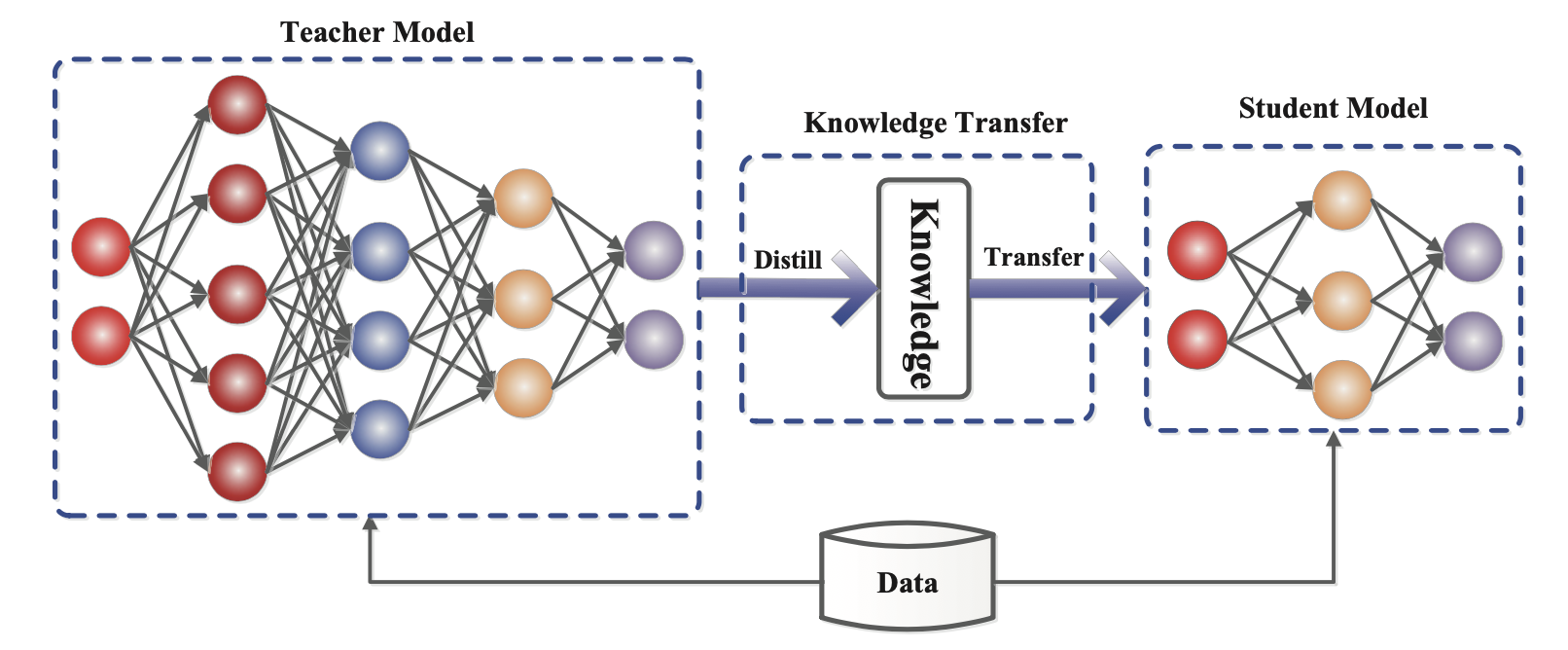
Given a dataset, the student is trained to match the teacher’s outputs using a distillation loss. In many neural networks, the output layer is a softmax; for example, an LLM produces a probability distribution over tokens. Let the logits immediately before the softmax be $\mathbf{z}_t$ for the teacher and $\mathbf{z}_s$ for the student. The distillation loss minimizes the discrepancy between the two softmax outputs under a high temperature $T$. When ground-truth labels $\mathbf{y}$ are available, the distillation objective can be combined with a supervised objective that compares the ground truth with the student’s soft logits (for example, cross-entropy).
where $\lambda$ is a hyperparameter that balances the soft and hard objectives. A common choice for $\mathcal{L}_\text{distll}$ is KL divergence / cross entropy.
An influential early example is DistilBERT (Sanh et al. 2019), which reduces BERT’s parameter count by 40% while retaining 97% of BERT’s performance on fine-tuned downstream tasks and running 71% faster. DistilBERT’s pre-training loss combines a soft distillation loss, a supervised training loss (i.e., Masked language modeling loss $\mathcal{L}_\text{MLM}$ for BERT), and a dedicated cosine embedding loss that aligns hidden-state vectors between teacher and student.
Distillation also combines naturally with quantization, pruning, or sparsification techniques: the teacher is the original full-precision dense model, while the student is quantized, pruned, or otherwise modified to achieve a higher sparsity level.
Quantization
Two widely used approaches exist for quantizing deep neural networks:
- Post-Training Quantization (PTQ): Train the model to convergence first, then convert weights to lower precision without additional training. This approach is usually inexpensive relative to training.
- Quantization-Aware Training (QAT): Apply quantization during pre-training or further fine-tuning. QAT typically delivers better performance, but it requires additional compute and access to representative training data.
It is important to distinguish theoretical best-case quantization strategies from what is practical given hardware kernel support. Because some matrix multiplication kernels are not supported on GPUs (e.g., INT4 x FP16), not every method described below yields real inference speedups in practice.
Challenges for Transformer Quantization
Many studies of transformer quantization report a consistent finding: a straightforward low-precision (e.g., 8-bit) post-training quantization can cause substantial performance degradation. The main culprit is the large dynamic range of activations, where naive activation quantization is not sufficient to preserve model capacity.
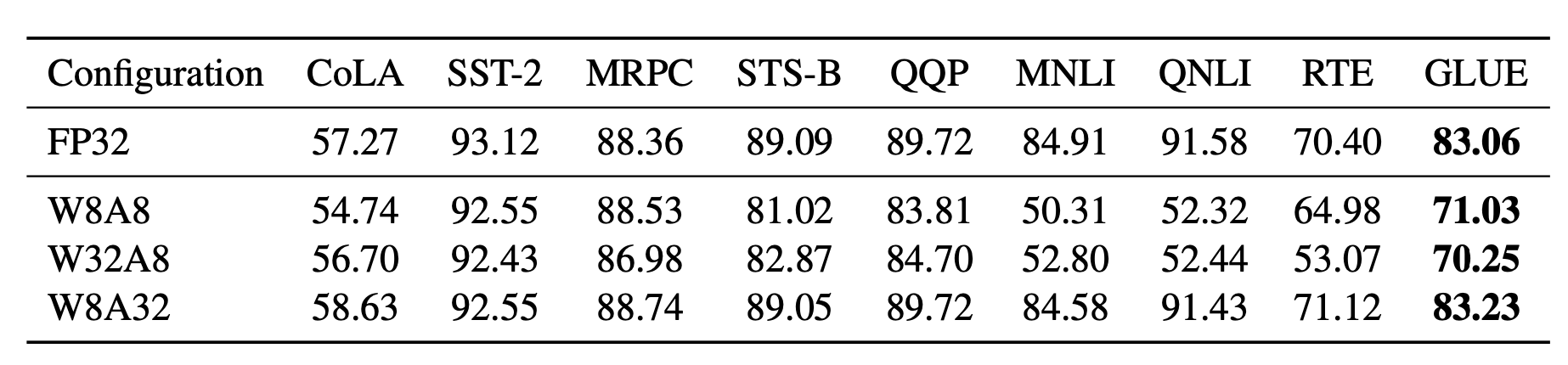
Bondarenko et al. (2021) observed, in a small BERT model, that the FFN input and output exhibit very different dynamic ranges due to strong outliers in the output tensor. As a result, per-tensor quantization applied to the FFN residual sum is likely to introduce noticeable error.
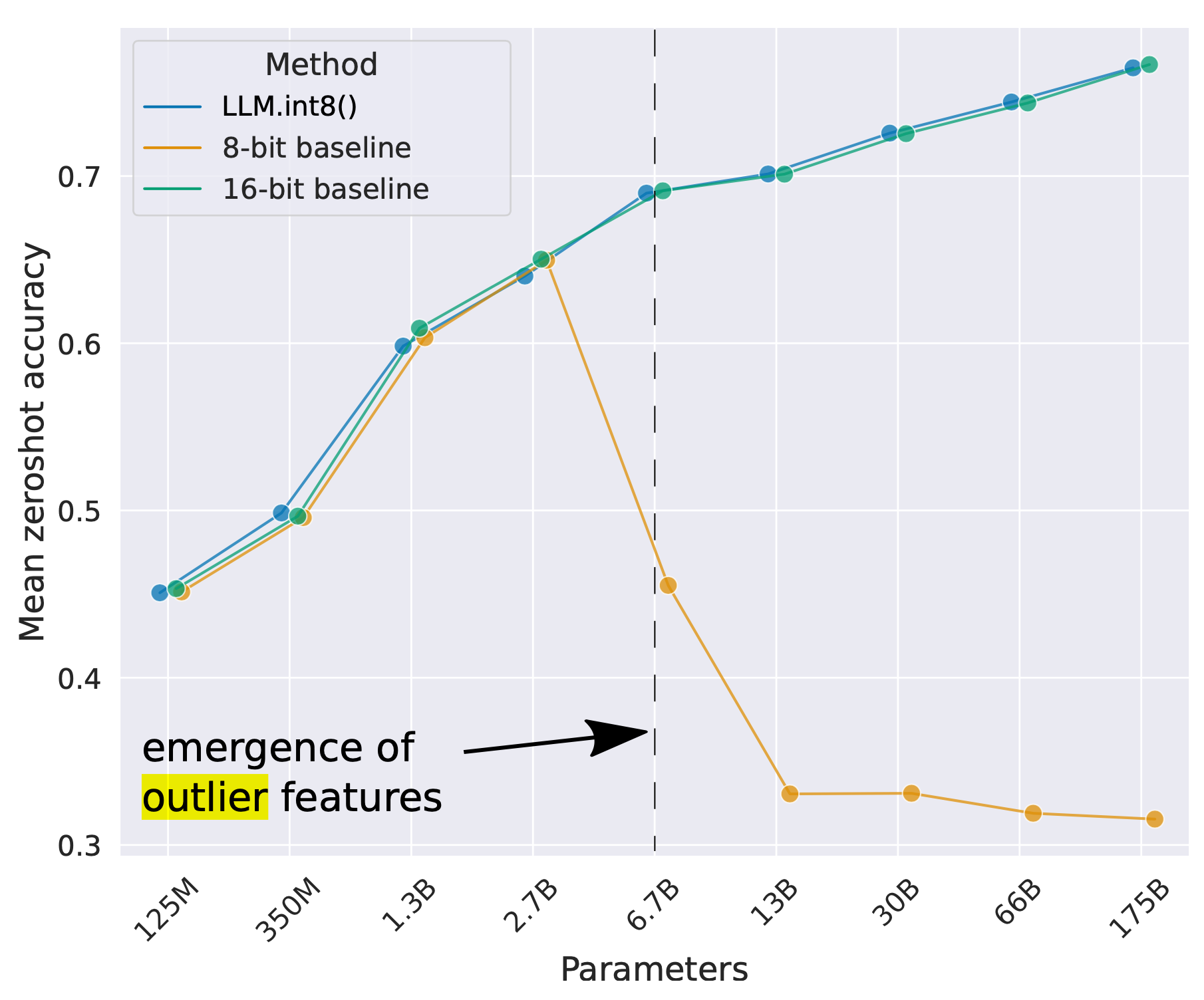
As model sizes scale to billions of parameters, high-magnitude outlier features begin to appear in all transformer layers, which can cause simple low-bit quantization methods to fail. Dettmers et al. (2022) reported this effect for OPT models larger than 6.7B parameters. Larger models have more layers with extreme outliers, and these outliers materially affect performance. In a few dimensions, activation outliers can be approximately 100× larger than most other values.
Post-training quantization (PTQ)
Mixed-precision quantization
The simplest way to address the quantization issues above is to quantize weights and activations at different precisions.
GOBO (Zadeh et al. 2020) was among the first to apply post-training quantization to transformers (specifically, a small BERT model). It assumes that each layer’s weights follow a Gaussian distribution and detects outliers by tracking the per-layer mean and standard deviation. Outlier values are retained in their original form, while the remaining values are assigned to multiple bins, and only the associated bin indices for the weights and the centroid values are stored.
Building on the finding that only particular activation layers in BERT (e.g., residual connections after the FFN) drive large performance drops, Bondarenko et al. (2021) used mixed-precision quantization by applying 16-bit quantization to problematic activations while using 8-bit quantization elsewhere.
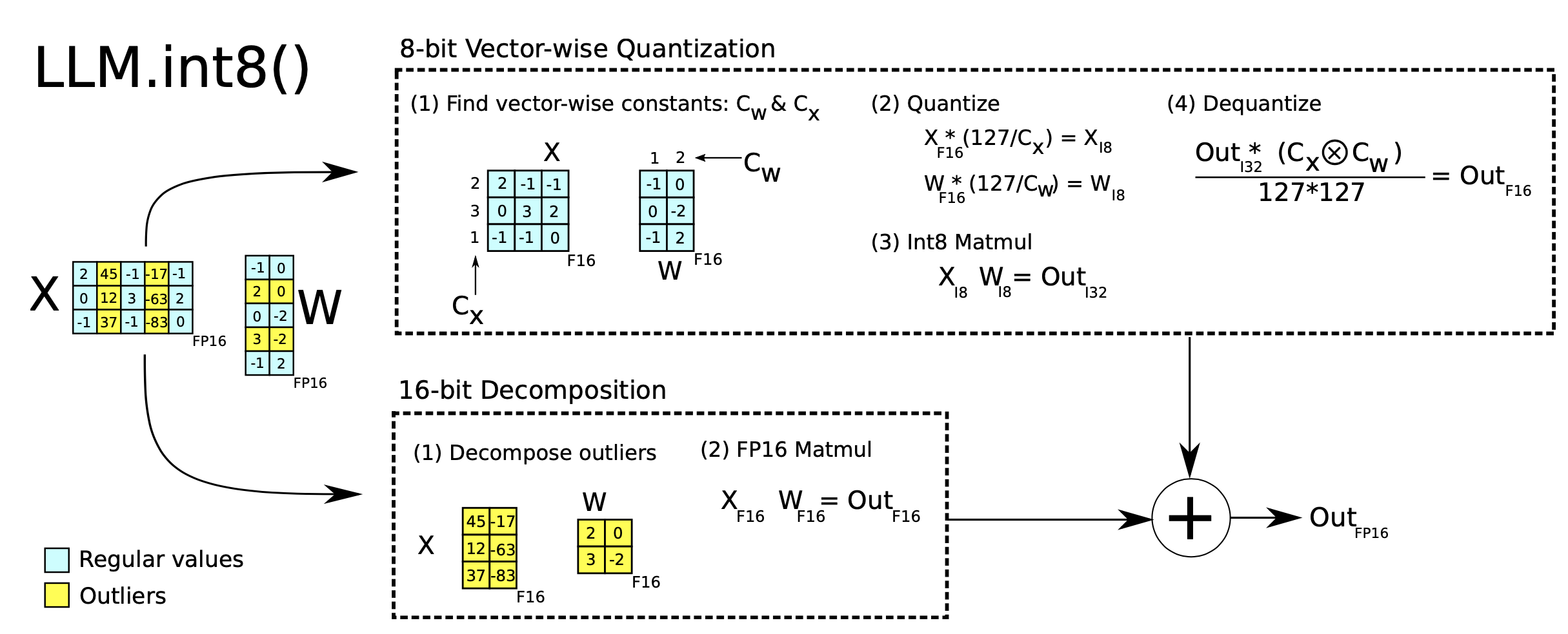
Mixed-precision quantization in LLM.int8() (Dettmers et al. 2022) is implemented with two mixed-precision decompositions:
- Matrix multiplication can be expressed as a set of independent inner products between row and column vectors, so quantization can be applied independently per inner product: each row and column is scaled by the absolution maximum values and then quantized to INT8.
- Outlier activation features (e.g., 20x larger than other dimensions) are kept in FP16, although they account for only a small fraction of the total weights. Outlier identification is empirical.
Quantization at fine-grained granularity
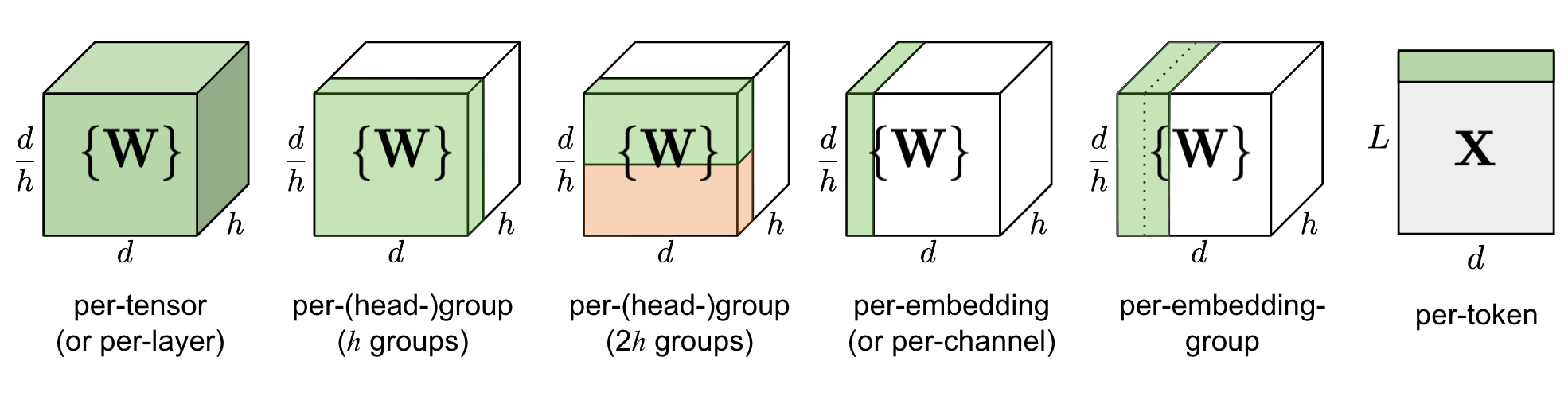
Quantizing an entire layer’s weight matrix as a single unit (often called “per-tensor” or “per-layer” quantization) is the easiest to implement, but it provides limited control over quantization granularity.
Q-BERT (Shen, Dong & Ye, et al. 2020) introduced group-wise quantization for a fine-tuned BERT model: it treats an individual matrix $W$ for each head in MHSA (multi-head self-attention) as a group, and then applies Hessian-based mixed-precision quantization.
Per-embedding group (PEG) activation quantization was motivated by the observation that outliers occur in only a small subset of the $d$ (hidden state / model size) dimensions (Bondarenko et al. 2021). While per-embedding quantization is computationally expensive, PEG splits the activation tensor into several equally sized groups along the embedding dimension, where all elements in the same group share quantization parameters. To ensure outliers are grouped together, PEG applies a deterministic, range-based permutation of embedding dimensions by sorting dimensions according to their value ranges.
ZeroQuant (Yao et al. 2022) adopts group-wise quantization for weights (as in Q-BERT) and token-wise quantization for activations. To avoid the overhead of quantization and de-quantization, ZeroQuant implements a custom kernel that fuses quantization with the preceding operator.
Second order information for quantization
Q-BERT (Shen, Dong & Ye, et al. 2020) proposed Hessian AWare Quantization (HAWQ) to support mixed-precision quantization. The key idea is that parameters associated with a larger Hessian spectrum (that is, larger top eigenvalues) are more sensitive to quantization error and therefore should be assigned higher precision. This is effectively an outlier identification mechanism.
From another perspective, quantization can be framed as an optimization problem. Given a weight matrix $\mathbf{W}$ and an input matrix $\mathbf{X}$ , the goal is to find a quantized weight matrix $\hat{\mathbf{W}}$ that minimizes the MSE:
$ \hat{\mathbf{W}}^* = {\arg\min}_{\hat{\mathbf{W}}} | \mathbf{W}\mathbf{X} - \hat{\mathbf{W}}\mathbf{X}| $
GPTQ (Frantar et al. 2022) views the weight matrix $\mathbf{W}$ as a set of row vectors ${\mathbf{w}}$ and quantizes each row independently. It iteratively quantizes additional weights selected greedily to minimize quantization error. For the selected weights, the update has a closed-form expression that leverages Hessian matrices. For additional details, see the paper and the OBQ (Optimal Brain Quantization; Frantar & Alistarh 2022) method. GPTQ can reduce OPT-175B weight precision to 3 or 4 bits with limited performance loss, but it applies only to weights, not activations.
Outlier smoothing
In transformer models, activations are generally more difficult to quantize than weights. SmoothQuant (Xiao & Lin 2022) introduced an approach that shifts outlier behavior from activations to weights using a mathematically equivalent transformation, enabling quantization of both weights and activations (W8A8). As a result, SmoothQuant is typically more hardware-efficient than mixed-precision quantization.
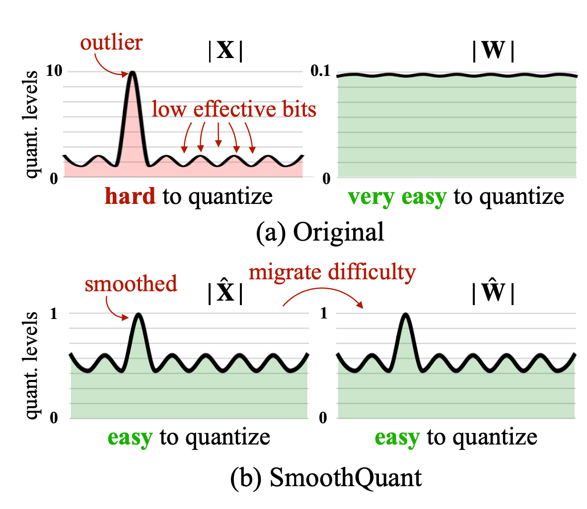
Given a per-channel smoothing factor $\mathbf{s}$, SmoothQuant rescales the weights as:
$ \mathbf{Y} = (\mathbf{X} \text{diag}(\mathbf{s})^{-1}) \cdot (\text{diag}(\mathbf{s})\mathbf{W}) = \hat{\mathbf{X}}\hat{\mathbf{W}} $
This smoothing factor can be fused offline into the parameters of preceding layers. A hyperparameter $\alpha$ controls the extent to which quantization difficulty is transferred from activations to weights: $\mathbf{s} = \max (\vert \mathbf{X}_j \vert)^\alpha / \max( \vert \mathbf{W}_j \vert )^{1-\alpha}$. The paper reports that $\alpha=0.5$ is a sweet spot for many LLMs in experiments. For models with more pronounced activation outliers, $\alpha$ can be increased.
Quantization-aware training (QAT)
Quantization-aware training incorporates quantization into pre-training or fine-tuning. It learns weights directly in low-bit representations and usually yields better performance, at the cost of additional training time and compute.
The most direct method is to fine-tune the quantized model on a training dataset that matches or is representative of the pre-training distribution. The objective can mirror pre-training (e.g., NLL/MLM for general language model training) or target a downstream task of interest (e.g., cross entropy for classification).
Another option is to treat the full-precision model as the teacher and the low-precision model as the student, then train the low-precision model using a distillation loss. Distillation typically does not require the original dataset; e.g., Wikipedia is a reasonable choice, and even random tokens can provide meaningful gains. Layer-by-layer Knowledge Distillation (LKD; Yao et al. 2022) quantizes the network layer by layer, using each layer’s original unquantized version as the teacher. For identical inputs, LKD minimizes the MSE between the multiplication using full-precision layer weights and the multiplication using the quantized layer weights.
Pruning
Network pruning reduces model size by removing model weights or connections deemed unimportant, ideally without reducing model capacity. Depending on the approach, pruning may or may not require retraining. Pruning methods are commonly categorized as unstructured or structured.
- Unstructured pruning can remove any weight or connection, so the original architecture is not preserved. It often maps poorly onto modern hardware, and therefore may not yield real inference speedups.
- Structured pruning seeks to preserve a dense-matrix-multiplication form with certain elements set to zero. To match hardware kernel constraints, structured sparsity may need to satisfy specific patterns. Here we focus on structured pruning for achieving high sparsity in transformer models.
A standard workflow for producing a pruned network consists of three steps:
- Train a dense network to convergence.
- Prune the network to remove the targeted structure.
- Optionally retrain the network to recover performance by learning new weights.
The idea that network pruning can reveal a sparse structure inside a dense model, where the resulting sparse network retains comparable performance, is closely related to the Lottery Ticket Hypothesis (LTH): a randomly initialized, dense, feed-forward network contains a collection of subnetworks, and only a subset of them (a sparse network) are “winning tickets” that can reach optimal performance when trained in isolation.
How to prune?
Magnitude pruning is one of the simplest and most effective approaches: it removes weights with the smallest absolute values. Some studies (Gale et al. 2019) report that simple magnitude pruning approaches can achieve comparable or better results than complicated pruning methods, such as variational dropout (Molchanov et al. 2017) and $l_0$ regularization (Louizos et al. 2017). Magnitude pruning scales well to large models and tends to deliver fairly consistent results across a broad range of hyperparameters.
Zhu & Gupta (2017) found that large sparse models can outperform smaller dense models. They introduced Gradual Magnitude Pruning (GMP), which increases a network’s sparsity progressively throughout training. At each training step, weights with the smallest absolute values are masked to zero to reach a target sparsity level $s$, and masked weights do not receive gradient updates during back-propagation. The target sparsity level $s$ increases as training proceeds. GMP is sensitive to the learning-rate schedule, which should be higher than the schedule used for dense training, but not so high that convergence is prevented.
Iterative pruning (Renda et al. 2020) repeats step 2 (prune) and step 3 (retrain) multiple times: each iteration prunes only a small fraction of weights, followed by retraining. This cycle continues until the desired sparsity is achieved.
How to retrain?
Retraining can be performed as straightforward fine-tuning on the same pre-training data or on other task-specific datasets.
The Lottery Ticket Hypothesis proposed weight rewinding as a retraining strategy: after pruning, the remaining weights are reinitialized back to the values they had earlier in training, and the model is retrained using the same learning-rate schedule.
Learning rate rewinding (Renda et al. 2020) resets only the learning rate to its earlier value, while the unpruned weights remain as they were at the end of the previous training stage. They observed that: (1) retraining with weight rewinding outperforms fine-tuning-based retraining across networks and datasets, and (2) learning-rate rewinding matches or outperforms weight rewinding in all evaluated scenarios.
Sparsity
Sparsity is an effective mechanism for increasing model capacity while keeping inference computationally efficient. For transformers, we consider two forms of sparsity:
- Sparsified dense layers, including both self-attention and FFN layers.
- Sparse model architectures, for example by incorporating Mixture-of-Experts (MoE) components.
N:M Sparsity via Pruning
N:M sparsity is a structured sparsity pattern that aligns well with modern GPU hardware optimizations: $N$ out of every $M$ consecutive elements are zeros. For example, Nvidia A100’s sparse tensor cores support 2:4 sparsity to accelerate inference (Nvidia 2020).
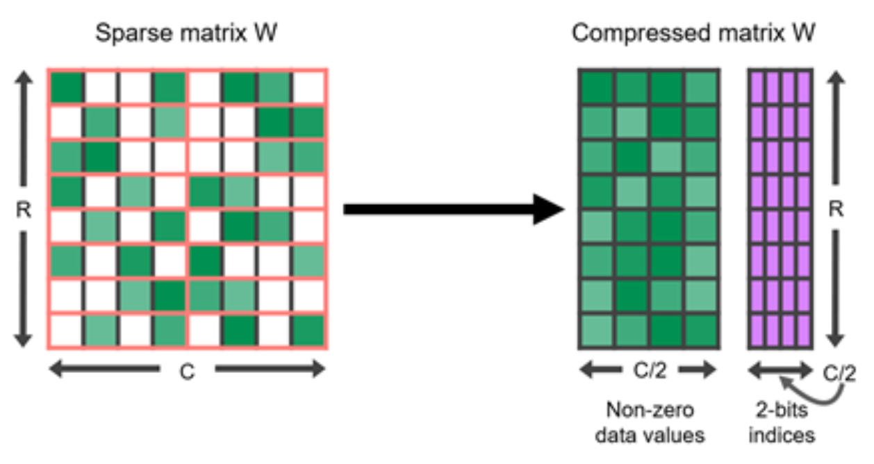
To sparsify a dense neural network so that it follows an N:M structured pattern, Nvidia (2020) recommends applying the three-step routine workflow for training a pruned network: train –> prune to satisfy 2:4 sparsity –> retrain.
Column permutation can expand the set of pruning choices, helping preserve large-magnitude parameters or satisfy constraints such as N:M sparsity (Pool & Yu 2021). As long as paired axes in the two matrices are permuted in the same order, the resulting matrix multiplication is unchanged. For example,
(1) In the self-attention module, if the same permutation is applied to axis 1 of the query embedding matrix $\mathbf{Q}$ and to axis 0 of the key embedding matrix $\mathbf{K}^\top$, the matrix multiplication result $\mathbf{Q}\mathbf{K}^\top$ remains unchanged.
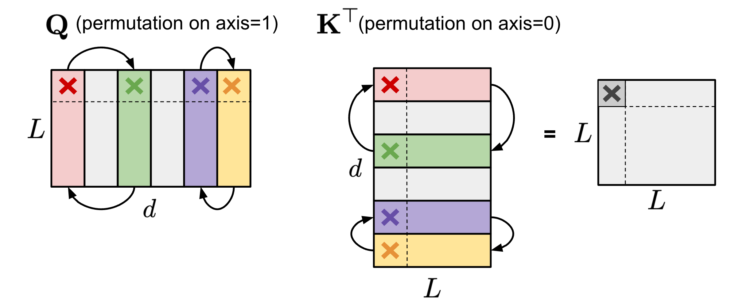
(2) In an FFN layer with two MLP layers and one ReLU non-linear layer, the first linear weight matrix $\mathbf{W}_1$ can be permuted along axis 1, and the second linear weight matrix $\mathbf{W}_2$ can be permuted along axis 0 using the same ordering.
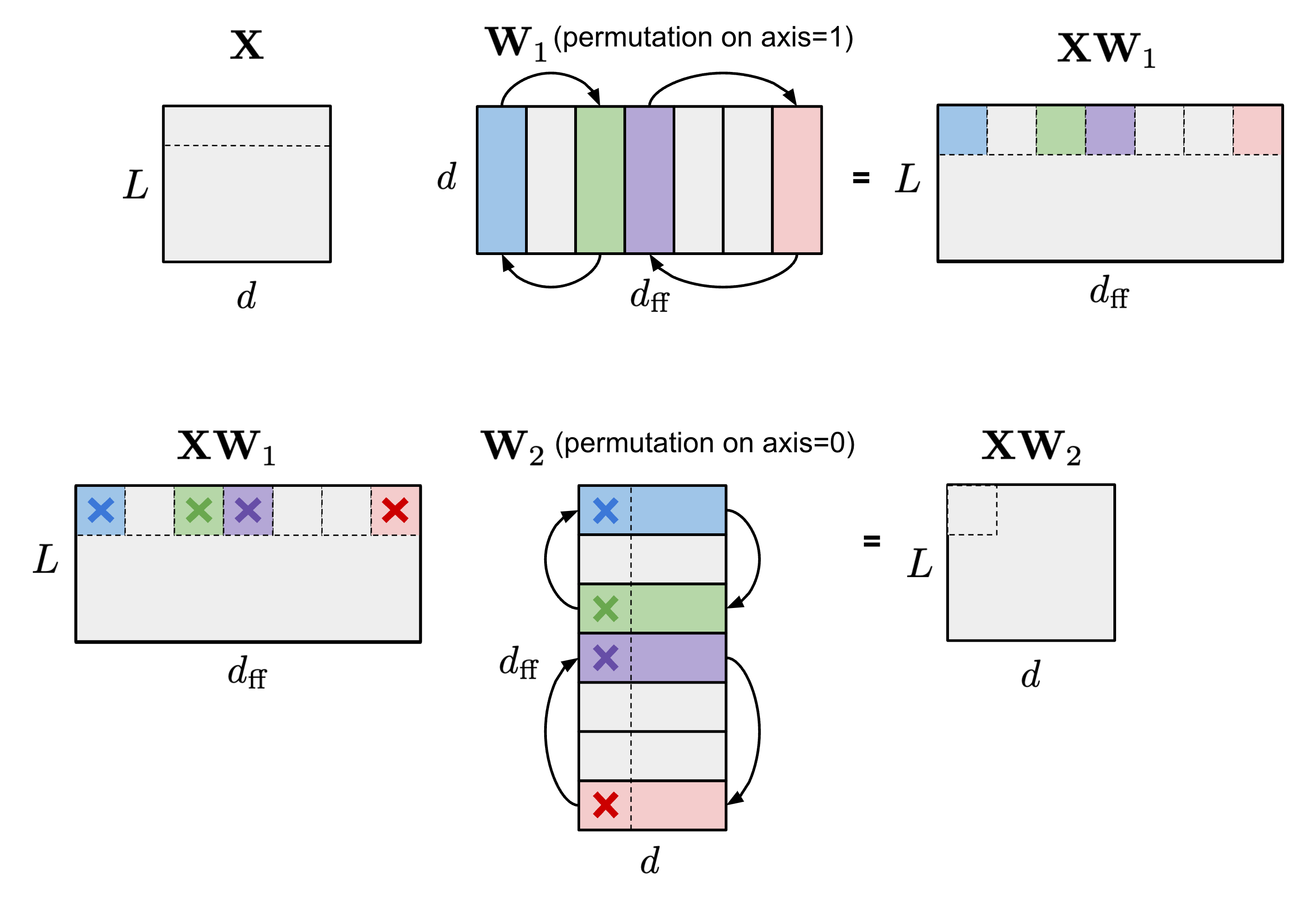
To enforce N:M structured sparsity, we can partition a matrix’s columns into multiple slides of $M$ columns (called a “stripe”). It is then straightforward to see that neither the ordering of columns within a stripe nor the ordering of the stripes affects the N:M sparsity constraint.
Pool & Yu (2021) introduced an iterative greedy algorithm for finding an optimal permutation that maximizes weight magnitude under N:M sparsity. The method speculatively swaps every pair of channels and then accepts only the single swap that yields the largest magnitude increase. That accepted swap defines a new permutation and completes one iteration. Because a greedy approach can become trapped in local minima, they proposed two techniques to escape them:
- Bounded regressions: In practice, two channels are randomly swapped up to a fixed number of times. The search depth is restricted to a single channel swap, which keeps the search space broad rather than deep.
- Narrow, deep search: Select multiple stripes and optimize them jointly.
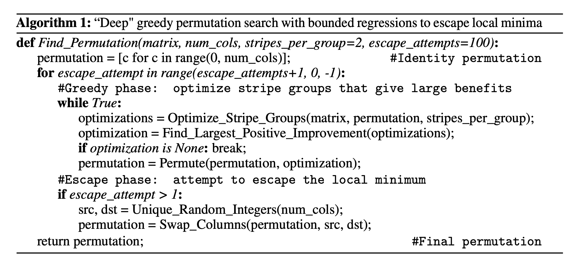
Compared with pruning a network in its default channel order, permuting the network prior to pruning can yield better performance.
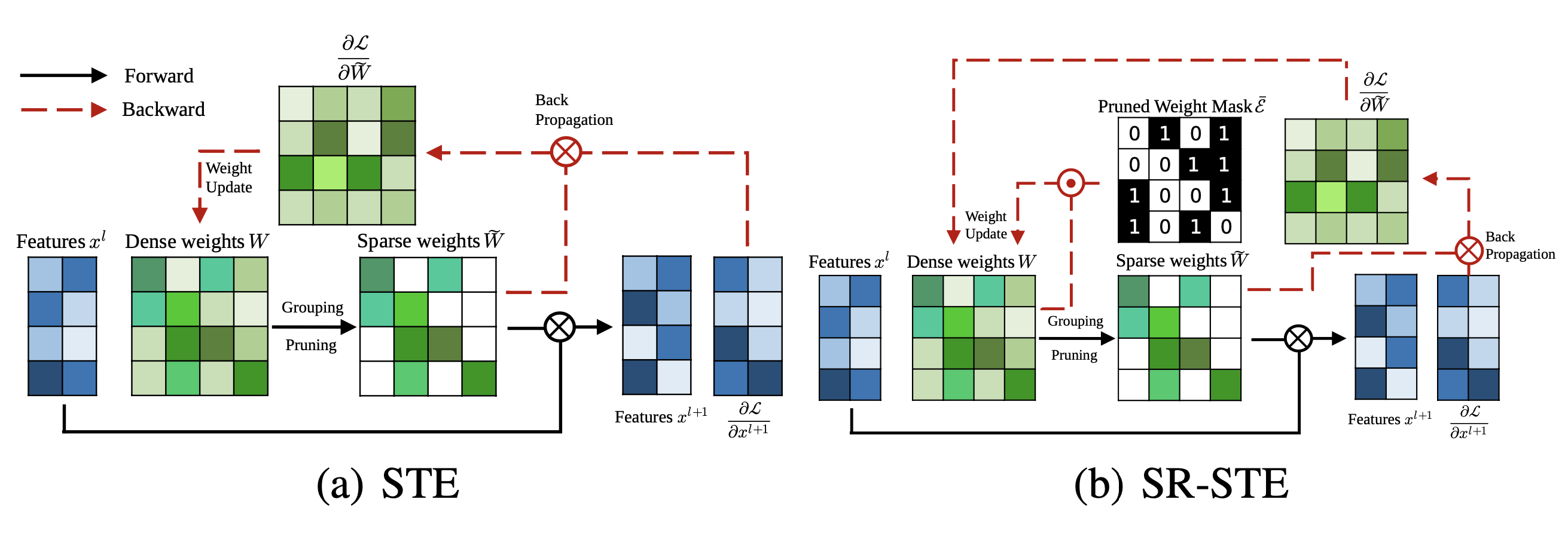
To train a model with N:M sparsity from scratch, Zhou & Ma, et al. (2021) extended STE (Straight-Through Estimator; Bengio et al. 2013), a technique commonly used for back-propagation updates in model quantization, so that it also applies to magnitude pruning and sparse parameter updates.
STE computes gradients of dense parameters with respect to the pruned network $\widetilde{W}$, $\partial \mathcal{L}/\partial \widetilde{W}$, and then applies them to the dense network $W$ as an approximation:
$ W_{t+1} \gets W_t - \gamma \frac{\partial\mathcal{L}}{\partial\widetilde{W}} $
The extended variant, SR-STE (Sparse-refined STE), updates the dense weights $W$ as follows:
$ W_{t+1} \gets W_t - \gamma \frac{\partial\mathcal{L}}{\partial\widetilde{W}} + \lambda_W (\bar{\mathcal{E}} \odot W_t) $ where $\bar{\mathcal{E}}$ is the mask matrix for $\widetilde{W}$, and $\odot$ denotes element-wise multiplication. SR-STE is designed to prevent large changes in the binary mask by: (1) constraining the values of weights pruned in $\widetilde{W}_t$, and (2) encouraging the non-pruned weights in $\widetilde{W}_t$.
Unlike STE or SR-STE, Top-KAST (Jayakumar et al. 2021) maintains constant sparsity throughout training in both the forward and backward passes, and it does not require forward passes with dense parameters or dense gradients.
At a single training step $t$, Top-KAST proceeds as follows:
- Sparse forward pass: Choose a subset of parameters $A^t \subset \Theta$ that contains, in each layer, the top-$K$ parameters by magnitude, constrained to the top $D$-proportion of weights. The parameterization $\alpha^t$ at time $t$ sets parameters to zero if they are not in $A^t$ (active weights).
where $\text{TopK}(\theta, x)$ selects the top $x$ proportion of weights from $\theta$ based on magnitude.
- Sparse backward pass: Next, apply gradients to a larger subset of parameters $B \subset \Theta$, where $B$ contains a $(D+M)$-proportion of weights and $A \subset B$. Updating a larger fraction of weights allows more effective exploration of alternative pruning masks, making it more likely to induce permutations among the top $D$-proportion of active weights.
Training is divided into two stages, and the additional coordinates in the set $B \setminus A$ determine how much exploration is introduced. The exploration level is expected to decrease gradually over training, and the mask eventually stabilizes.
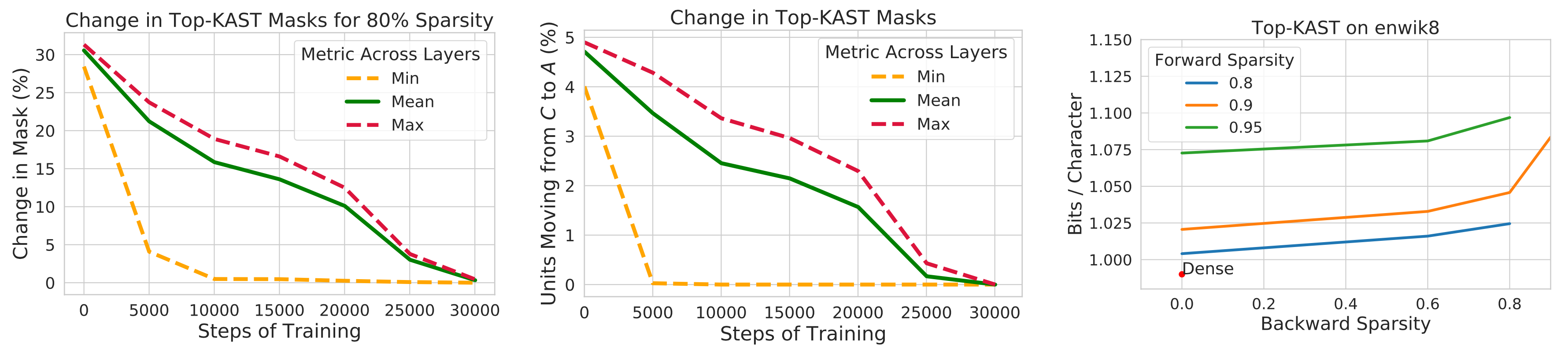
To mitigate the rich-get-richer effect, Top-KAST penalizes the magnitude of active weights using an L2 regularization term, encouraging greater exploration of new items. Parameters in $B \setminus A$ receive a stronger penalty than those in $A$, raising the selection threshold during updates to help stabilize the mask.
Sparsified Transformer
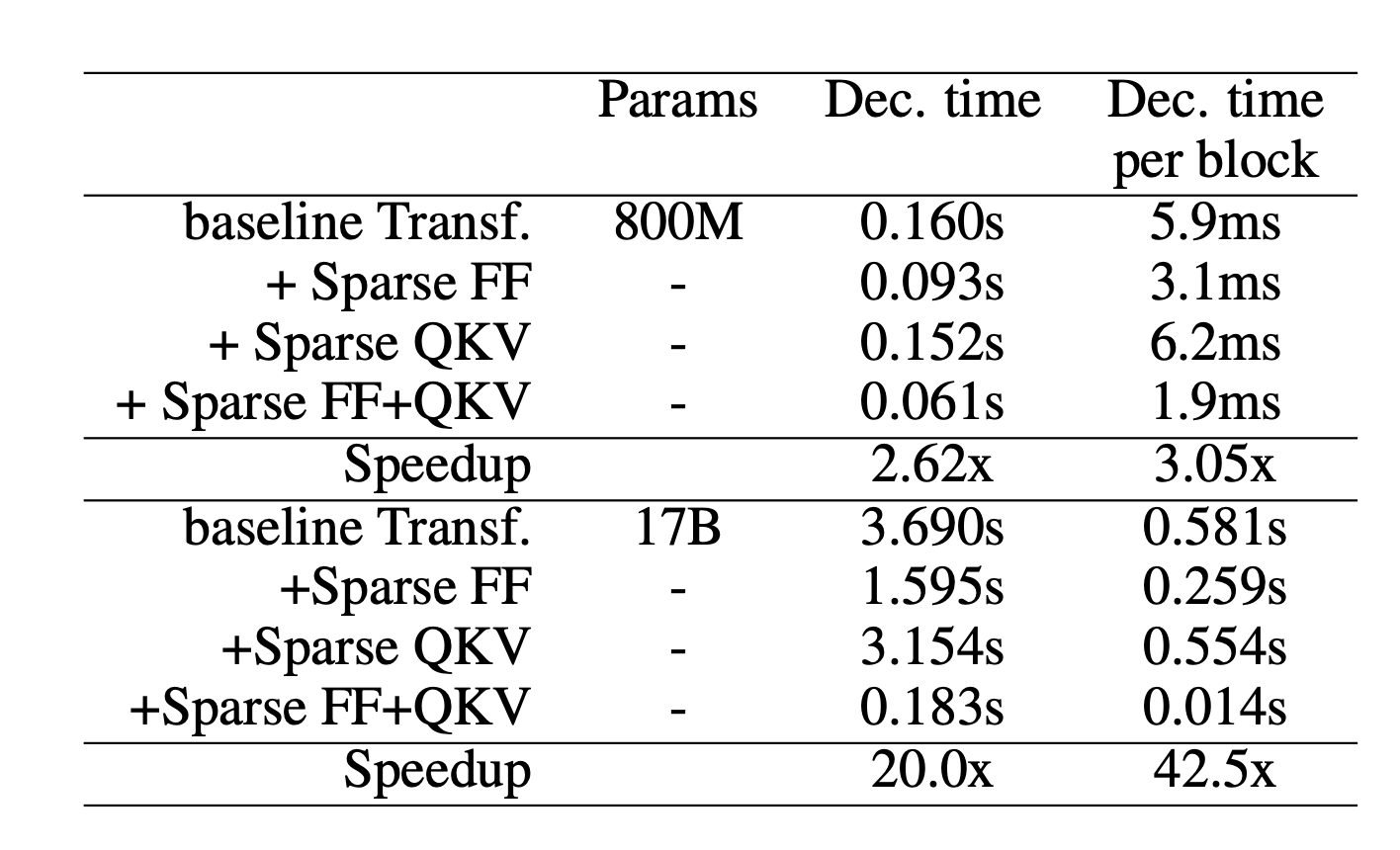
Scaling Transformer (Jaszczur et al. 2021) sparsifies both self-attention and FFN layers in the transformer architecture, delivering a 37x speedup for single-example inference.
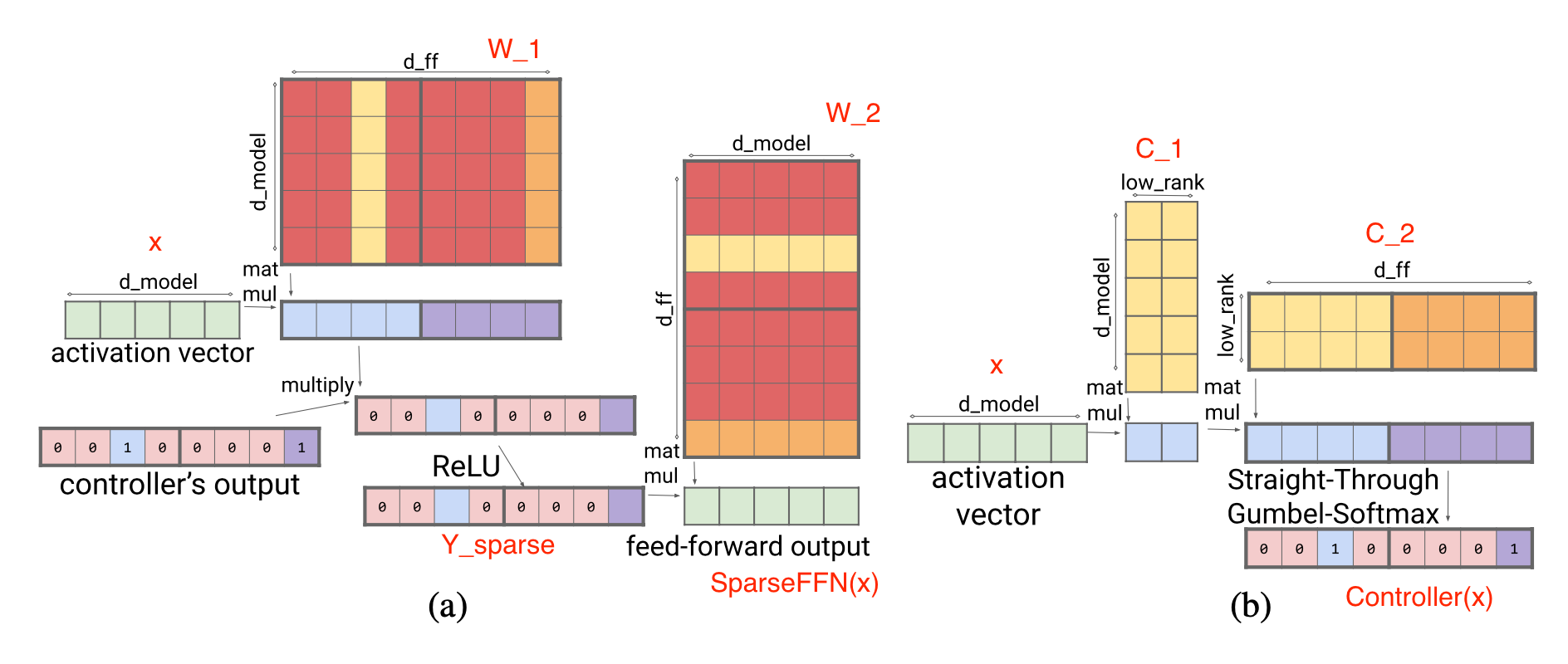
Sparse FFN layer: Each FFN layer includes two MLPs with a ReLU in between. Since ReLU introduces many zeros, they impose a fixed activation structure that enforces exactly one non-zero value per block of $N$ elements. The sparsity pattern is dynamic and varies by token.
Here, each activation in $Y_\text{sparse}$ maps to one column in $W_1$ and one row in $W_2$. The controller is implemented as a low-rank bottleneck dense layer, $C_1 \in \mathbb{R}^{d_\text{model} \times d_\text{lowrank}}, C_2 \in \mathbb{R}^{d_\text{lowrank} \times d_\text{ff}}$ and $d_\text{lowrank} = d_\text{model} / N$. For inference, it uses $\arg\max$ to choose which columns are non-zero, while during training it relies on the Gumbel-softmax trick (Jang et al. 2016). Because $\text{Controller}(x)$ can be computed before loading the FFN weight matrices, the implementation can determine which columns will be zeroed out and therefore avoid loading them into memory, improving inference speed.
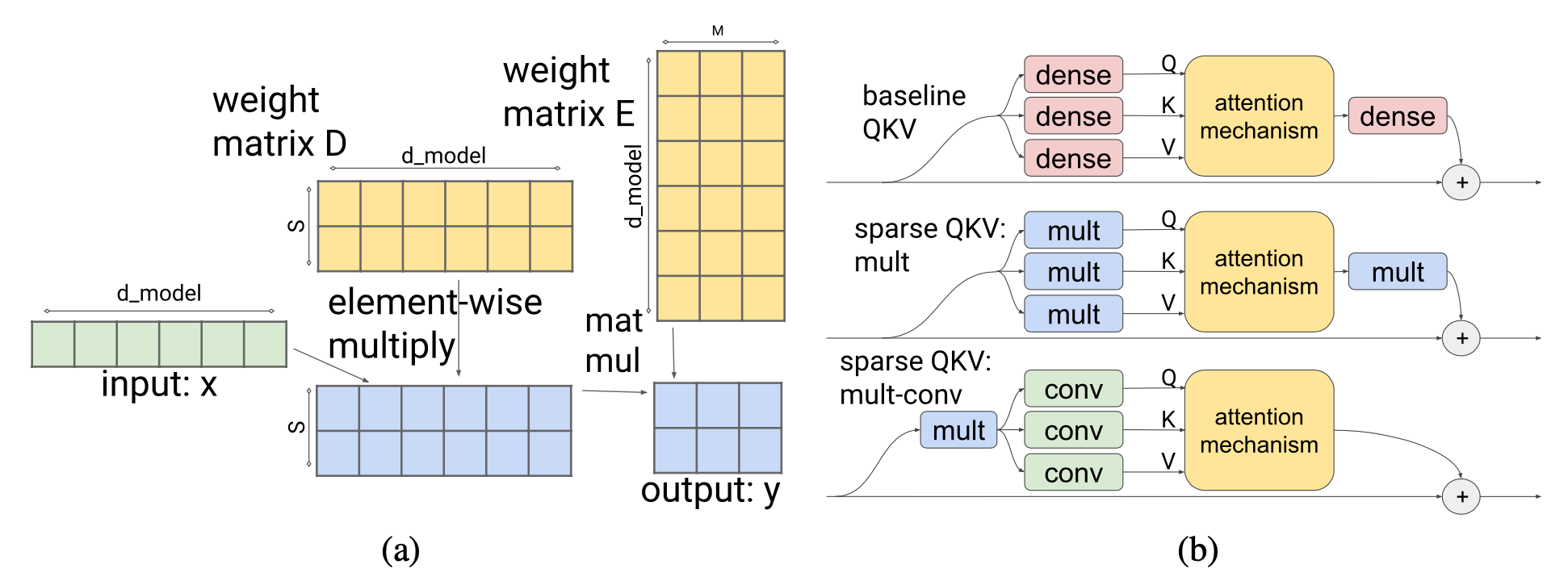
Sparse QKV (attention) layer: In the attention layer, the dimensionality $d_\text{model}$ is partitioned into $S$ modules, each with size $M=d_\text{model} /S$. To ensure that each partition can access any portion of the embedding, Scaling Transformer adds a multiplicative layer (that is, a layer that multiplies inputs element-wise from multiple neural network layers). This layer can represent an arbitrary permutation while using fewer parameters than a dense layer.
Given an input vector $x \in \mathbb{R}^{d_\text{model}}$, the multiplicative layer produces $y \in \mathbb{R}^{S \times M}$:
The multiplicative-layer output is a tensor with size $\in \mathbb{R}^{\text{batch size}\times \text{length} \times S \times M}$. This tensor is then passed through a two-dimensional convolutional layer, where $\text{length}$ and $S$ are interpreted as the height and width of an image. This convolution further reduces both parameter count and the computation time of the attention layer.
To better support long sequences, Scaling Transformer additionally incorporates LSH (locality-sensitive hashing) attention from Reformer (Kitaev, et al. 2020) and FFN block recurrence, producing Terraformer.
Mixture-of-Experts
Mixture-of-experts (MoE) models rely on a set of “expert” networks, and each example activates only a subset of them to generate predictions. The concept dates back to the 1990s (Jacobs et al. 1991) and is closely related to ensemble methods. For details on incorporating MoE modules into transformers, see my previous post on large model training techniques and the MoE survey by Fedus et al. 2022.
With an MoE architecture, decoding uses only a fraction of the parameters, reducing inference cost. The capacity of each expert is controlled by a hyperparameter, capacity factor $C$, and expert capacity is defined as:
where top-$k$ experts are selected per token. A larger $C$ increases expert capacity and improves performance, but also increases computational cost. When $C>1$, slack capacity is added; otherwise, when $C<1$, the routing network must ignore some tokens.
Routing Strategy Improvement
An MoE layer includes a routing network that assigns a subset of experts to each input token. In vanilla MoE models, tokens are routed to preferred experts in their natural sequence order. If a token is assigned to experts that have already reached capacity, the token is marked as “overflowed” and skipped.
V-MoE (Vision MoE; Riquelme et al. 2021) inserts MoE layers into ViT (Vision Transformer). It matches prior state-of-the-art performance while requiring only half the inference compute. V-MoE can scale to 15B parameters. In their experiments, they used $k=2$, 32 experts, and every-2 expert placement (meaning MoE layers are placed in every other layer).
Because expert capacity is limited, important and informative tokens can be discarded if they appear too late in a predefined order (for example, word order in a sentence, or patch order in an image). To address this limitation of vanilla routing, V-MoE uses BPR (Batch Priority Routing), which assigns experts to tokens with higher priority scores first. BPR computes a priority score per token (max or sum of the top-$k$ router scores) prior to expert assignment, and then reorders tokens accordingly. This ensures that the expert capacity buffer is filled with key tokens first.
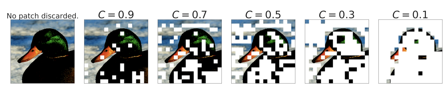
BPR significantly outperforms vanilla routing when $C\leq 0.5$, where the model begins dropping a substantial number of tokens. It enables the model to remain competitive with a dense network even at relatively low capacities.
When examining how to interpret class-to-expert associations for images, they found that early MoE layers are more general, while later MoE layers can specialize in a small number of image classes.
Task MoE (Task-level Mixture-of-Experts; Kudugunta et al. 2021 ) incorporates task information and routes tokens at the task level rather than the word or token level for machine translation. Using MNMT (multilingual neural machine translation) as an example, they group translation tasks based on target language or language pairs.
Token-level routing is dynamic, and routing decisions are made independently per token. As a result, at inference time the server must preload all experts. In contrast, task-level routing is static for a fixed task, so an inference server for a given task only needs to preload $k$ experts (assuming top-$k$ routing). According to their experiments, Task MoE achieves performance gains similar to token-level MoE relative to a dense baseline, while providing 2.6x higher peak throughput and using 1.6% of the decoder size.
In essence, task-level MoE categorizes a task distribution using predefined heuristics and injects this human knowledge into the router. When such heuristics are unavailable (for example, in a general sentence continuation task), applying Task MoE is not straightforward.
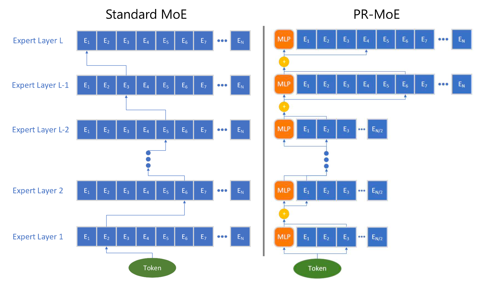
PR-MoE (Pyramid residual MoE; Rajbhandari et al. 2022) routes each token through one fixed MLP and one selected expert. Motivated by the observation that MoE is more beneficial in later layers, PR-MoE allocates more experts to later layers. The DeepSpeed library provides flexible multi-expert, multi-data parallelism to support training PR-MoE with varying numbers of experts across layers.
Kernel Improvement
Expert networks may be distributed across devices. However, as the number of GPUs increases, the number of experts per GPU decreases, while all-to-all communication between experts becomes more expensive. All-to-all communication across GPUs relies on NCCL P2P APIs, which cannot saturate the bandwidth of high-speed links (for example, NVLink, HDR InfiniBand) at large scale because each individual chunk becomes smaller as more nodes participate. The standard all-to-all algorithm therefore performs poorly at scale when the workload per node is small. Multiple kernel-level improvements have been proposed to make MoE computation more efficient, including approaches that reduce the cost and latency of all-to-all communication.
Both the DeepSpeed library (Rajbhandari et al. 2022) and TUTEL (Hwang et al. 2022) implement a tree-based hierarchical all-to-all algorithm that performs an intra-node all-to-all followed by an inter-node all-to-all. This reduces the number of communication hops from $O(G)$ to $O(G_\text{node} + G / G_\text{node})$, where $G$ is the total number of GPU nodes and $G_\text{node}$ is the number of GPU cores per node. Although this approach doubles the communication volume, it scales better for small batches at large scale because, at small batch sizes, latency rather than bandwidth becomes the dominant bottleneck.
DynaMoE (Kossmann et al. 2022) applies dynamic recompilation to match computational resources to experts’ dynamic workloads. The RECOMPILE mechanism recompiles the computation graph from scratch and reallocates resources only when necessary. It tracks the number of samples routed to each expert and dynamically adjusts their capacity factors $C$ to reduce memory and computation requirements at runtime. Based on the observation that sample-to-expert assignments converge early in training, it introduces sample assignment caching after convergence, and then uses RECOMPILE to remove the dependency between the gating network and experts.
Architectural Optimization
The survey on Efficient Transformers (Tay et al. 2020) reviews a range of transformer architectures designed for improved computational and memory efficiency. It is highly recommended. You may also refer to my post “The Transformer Family Version 2.0” for an in-depth overview of many transformer architecture improvements, including modifications that reduce runtime cost.
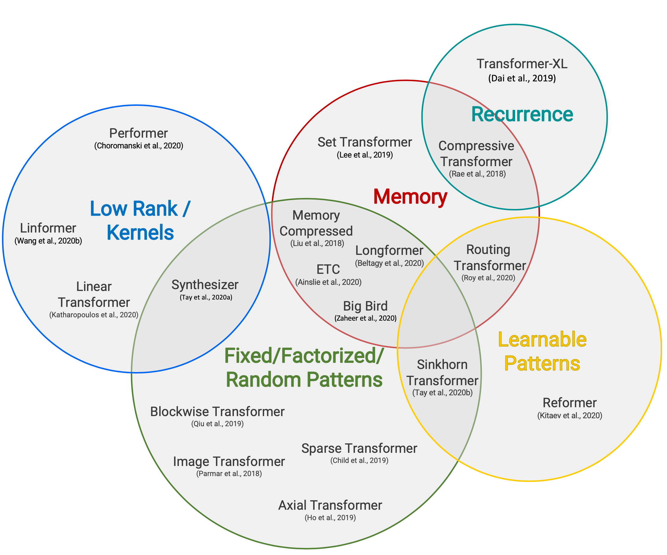
(Image source: Tay et al. 2020)
Because self-attention has quadratic time and memory complexity, it is the primary bottleneck for more efficient transformer decoding. Accordingly, efficient transformer variants apply some form of sparsity to an otherwise dense attention layer. The following provides only a high-level overview, with several items derived from Tay et al. 2020.
Sparse Attention Patterns
-
Fixed Patterns restrict the attention matrix’s field of view using predefined, fixed layouts.
- Chunk input sequences into fixed blocks, such as Blockwise Attention;
- Image Transformer uses local attention;
- Sparse Transformer uses strided attention patterns.
-
Combined Patterns learn to sort or cluster input tokens, enabling a more optimal global view of the sequence while preserving the efficiency benefits of fixed patterns.
- Sparse Transformer combines strided and local attention;
- Given a high-dimensional input tensor, rather than applying attention to a flattened representation, Axial Transformer applies multiple attention operations, each along a single axis of the input tensor.
- ETC, Longformer and Big Bird combines local and global context, as well as strided or random attention.
-
Learnable Patterns learn to identify an effective attention pattern.
- Reformer clusters tokens into clusters based on hash-based similarity (LSH);
- Routing Transformer runs $k$-means clustering on tokens;
- Sinkhorn Sorting Network learns to sort blocks of the input sequence.
Recurrence
Recurrence connects multiple blocks or segments through a recurrence mechanism.
- Transformer-XL uses longer context by reusing hidden states across segments.
- Universal Transformer combines self-attention with the recurrent mechanism in RNN.
- Compressive Transformer extends Transformer-XL with additional memory, including a set of memory slots for past activiations and compressive memory slots for compressed activations. When the model receives a new input segment, the oldest activations in primary memory are moved into compressed memory, where a compression function is applied.
Memory Saving Designs
Memory-saving designs are architectural changes intended to reduce memory usage.
- Linformer projects the length dimension of keys and values into a lower-dimensional representation ($N \to k$), reducing memory complexity from $N \times N$ to $N \times k$.
- Shazeer (2019) proposed multi-query attention, in which keys and values are shared across different attention heads, substantially reducing tensor sizes and memory cost.
- Random feature attention and Performer use kernel methods to obtain a cheaper mathematical formulation of self-attention.
Adaptive Attention
Adaptive attention allows the model to learn an optimal attention span, or to decide when to exit computation early, depending on the input tokens.
- Adaptive Attention Span trains the model to learn the optimal attention span per token per head via a soft mask between the token and other keys.
- Universal Transformer incorporates a recurrent mechanism and uses ACT (Adaptive computation time) to dynamically determine the number of recurrent steps.
- Depth-Adaptive Transformer and CALM learn when to exit early from computation layers per token using confidence measures, achieving favorable performance-efficiency tradeoffs.
Citation
Cited as:
Weng, Lilian. (Jan 2023). Large Transformer Model Inference Optimization. Lil’Log. https://lilianweng.github.io/posts/2023-01-10-inference-optimization/.
Or
@article{weng2023inference,
  title   = "Large Transformer Model Inference Optimization",
  author  = "Weng, Lilian",
  journal = "Lil'Log",
  year    = "2023",
  month   = "Jan",
  url     = "https://lilianweng.github.io/posts/2023-01-10-inference-optimization/"
}
References
[1] Bondarenko et al. “Understanding and overcoming the challenges of efficient transformer quantization” ACL 2021.
[2] Dettmers et al. “LLM.int8(): 8-bit Matrix Multiplication for Transformers at Scale” NeuriPS 2022
[3] Zadeh et al. “Gobo: Quantizing attention-based NLP models for low latency and energy efficient inference.” MICRO 2020
[4] Shen, Dong & Ye, et al. “Q-BERT: Hessian based ultra low precision quantization of BERT” AAAI 2020.
[5] Yao et al. “ZeroQuant: Efficient and affordable post-training quantization for large-scale transformers” arXiv preprint arXiv:2206.01861 (2022).
[6] Frantar et al. “GPTQ: Accurate Quantization for Generative Pre-trained Transformers” arXiv preprint arXiv:2210.17323 (2022).
[7] Xiao & Lin “SmoothQuant: Accelerated sparse neural training: A provable and efficient method to find N:M transposable masks.” arXiv preprint arXiv:2211.10438 (2022). | code
[8] Pool & Yu. “Channel Permutations for N:M Sparsity.” NeuriPS 2021. | code
[9] Zhou & Ma, et al. “Learning N:M fine-grained structured sparse neural networks from scratch.” arXiv preprint arXiv:2102.04010 (2021).
[10] Jayakumar et al. “Top-KAST: Top-K Always Sparse Training.” NeuriPS 2020.
[11] Nvidia. “Nvidia A100 tensor core GPU architecture.” 2020.
[12] Gale, Elsen & Hooker. “The State of Sparsity in Deep Neural Networks.” arXiv preprint arXiv:1902.09574 (2019).
[13] Zhu & Gupta. “To Prune, or Not to Prune: Exploring the Efficacy of Pruning for Model Compression.” arXiv preprint arXiv:1710.01878 (2017).
[14] Renda et al. “Comparing rewinding and fine-tuning in neural network pruning.” arXiv preprint arXiv:2003.02389 (2020).
[15] Zhou & Ma, et al. “Learning N:M fine-grained structured sparse neural networks from scratch.” arXiv preprint arXiv:2102.04010 (2021).
[16] Pool & Yu. “Channel Permutations for N:M Sparsity.” NeuriPS 2021. | code
[17] Jaszczur et al. “Sparse is Enough in Scaling Transformers.” NeuriPS 2021.
[18] Mishra et al. “An Survey of Neural Network Compression.” arXiv preprint arXiv:1710.09282 (2017).
[19] Fedus et al. “A Review of Sparse Expert Models in Deep Learning.” arXiv preprint arXiv:2209.01667 (2022)..
[20] Riquelme et al. “Scaling vision with sparse mixture of experts.” NeuriPS 2021.
[21] Kudugunta et al. “Beyond Distillation: Task-level Mixture-of-Experts for Efficient Inference.” arXiv preprint arXiv:2110.03742 (2021).
[22] Rajbhandari et al. “DeepSpeed-MoE: Advancing mixture-of-experts inference and training to power next-generation ai scale.” arXiv preprint arXiv:2201.05596 (2022).
[23] Kossmann et al. “Optimizing mixture of experts using dynamic recompilations.” arXiv preprint arXiv:2205.01848 (2022).
[24] Hwang et al. “Tutel: Adaptive mixture-of-experts at scale.” arXiv preprint arXiv:2206.03382 (2022). | code
[25] Noam Shazeer. “Fast Transformer Decoding: One Write-Head is All You Need.” arXiv preprint arXiv:1911.02150 (2019).
[26] Tay et al. “Efficient Transformers: A Survey.” ACM Computing Surveys 55.6 (2022): 1-28.
[27] Pope et al. “Efficiently Scaling Transformer Inference.” arXiv preprint arXiv:2211.05102 (2022).
[28] Frankle & Carbin. “The Lottery Ticket Hypothesis: Finding Sparse, Trainable Neural Networks.” ICLR 2019.
[29] Elabyad et al. “Depth-Adaptive Transformer.” ICLR 2020.
[30] Schuster et al. “Confident Adaptive Language Modeling.” arXiv preprint arXiv:2207.07061 (2022).
[31] Gou et al. “https://arxiv.org/abs/2006.05525” arXiv preprint arXiv:2006.05525 (2020).
[32] Hinton et al. “Distilling the Knowledge in a Neural Network.” NIPS 2014.
[33] Sanh et al. “DistilBERT, a distilled version of BERT: smaller, faster, cheaper and lighter.” Workshop on Energy Efficient Machine Learning and Cognitive Computing @ NeuriPS 2019.