This is Part 3 in the series on learning with insufficient data (previous installments: Part 1 and Part 2). Here, we examine two broad strategies for creating synthetic training data.

• Augmented data. Starting from an existing set of training samples, we apply augmentations, distortions, or transformations to generate additional examples while preserving the essential attributes. A range of augmentation methods for text and images was covered in a previous post on contrastive learning. For completeness, I reproduce that data-augmentation section here, with minor edits.
• New data. When only a few examples, or even none, are available, we can use powerful pretrained models to generate entirely new examples. This has become especially practical in recent years given rapid progress in large pretrained language models (LM). Few-shot prompting has been shown to work well for enabling LMs to learn in context without additional training.

Data Augmentation

Data augmentation aims to modify the input form (for example, text phrasing or visual appearance) while keeping the underlying semantic meaning unchanged.

Image Augmentation

Basic Image Processing Operations

There are many ways to alter an image while preserving its semantic content. Any single augmentation, or a composition of several operations, can be used.

• Randomly crop, then resize back to the original dimensions.
• Random color distortion.
• Random Gaussian blur.
• Random color jitter.
• Random horizontal flip.
• Random grayscale conversion.
• And many others. See PIL.ImageOps for ideas.

Task-Specific Augmentation Strategies

When the downstream task is known, it can be beneficial to learn an optimal augmentation policy (that is, which operations to apply and how to sequence them) in order to maximize downstream performance.

• AutoAugment (Cubuk, et al. 2018) is motivated by neural architecture search. It formulates the search for effective image-classification augmentations (for example, shearing, rotation, invert, etc.) as an RL problem, and it searches for the combination that yields the highest evaluation-set accuracy. AutoAugment can also be run in an adversarial manner (Zhang, et al 2019).
• RandAugment (Cubuk et al., 2019) substantially simplifies AutoAugment by shrinking the search space. It controls the magnitudes of multiple transformation operations using a single magnitude parameter.
• Population based augmentation (PBA; Ho et al., 2019) merges PBT (“population based training”; Jaderberg et al, 2017) with AutoAugment, using an evolutionary approach to train a population of child models in parallel and evolve strong augmentation strategies.
• Unsupervised Data Augmentation (UDA; Xie et al., 2019) chooses, from a set of candidate augmentation strategies, a subset that minimizes the KL divergence between the predicted distribution for an unlabeled example and that of its unlabeled augmented counterpart.

Image Mixture

Image-mixture techniques construct new training examples by combining existing samples.

• Mixup (Zhang et al., 2018) performs a global mixture by producing a weighted, pixel-wise combination of two existing images $I_1$ and $I_2$: $I_\text{mixup} \gets \alpha I_1 + (1-\alpha) I_2$ and $\alpha \in [0, 1]$.
• Cutmix (Yun et al., 2019) performs a region-level mixture by creating a new example that uses a local region from one image and the remainder from another. $I_\text{cutmix} \gets \mathbf{M}_b \odot I_1 + (1-\mathbf{M}_b) \odot I_2$, where $\mathbf{M}_b \in \{0, 1\}^I$ is a binary mask and $\odot$ denotes element-wise multiplication. This is equivalent to filling the cutout (DeVries & Taylor 2017) region with the corresponding region from a different image.
• Given a query $\mathbf{q}$, MoCHi (“mixing of contrastive hard negatives”; Kalantidis et al. 2020) maintains a queue of $K$ negative features $Q={\mathbf{n}_1, \dots, \mathbf{n}_K }$ and sorts them by similarity to the query, $\mathbf{q}^\top \mathbf{n}$, in descending order. The first $N$ items are treated as the hardest negatives, $Q^N$. Synthetic hard examples can then be generated by $\mathbf{h} = \tilde{\mathbf{h}} / |\tilde{\mathbf{h}}|_2$ where $\tilde{\mathbf{h}} = \alpha\mathbf{n}_i + (1-\alpha) \mathbf{n}_j$ and $\alpha \in (0, 1)$. Even harder examples can be produced by mixing with the query feature, $\mathbf{h}’ = \tilde{\mathbf{h}’} / |\tilde{\mathbf{h}’}|_2$ where $\tilde{\mathbf{h}’} = \beta\mathbf{q} + (1-\beta) \mathbf{n}_j$ and $\beta \in (0, 0.5)$.

Text Augmentation

Lexical Edits

Easy Data Augmentation (EDA; Wei & Zou 2019) specifies a small set of straightforward yet effective text-augmentation operations. Given a sentence, EDA randomly selects and applies one of the following four operations:

1. Synonym replacement (SR): Replace $n$ random non-stop words with their synonyms.
2. Random insertion (RI): Insert a random synonym of a randomly chosen non-stop word into the sentence at a random position.
3. Random swap (RS): Randomly swap two words, repeated $n$ times.
4. Random deletion (RD): Delete each word independently with probability $p$.

where $p=\alpha$ and $n=\alpha \times \text{sentence_length}$, motivated by the intuition that longer sentences can tolerate more noise while still preserving the original label. The hyperparameter $\alpha$ approximately represents the fraction of words in a sentence that a single augmentation may modify.

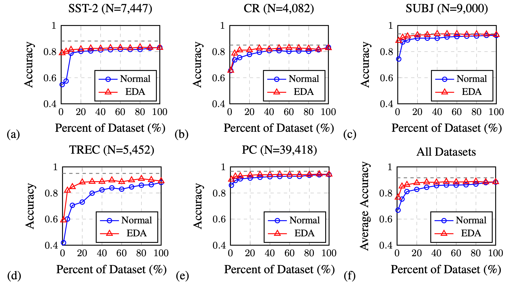
EDA is reported to increase classification accuracy across multiple benchmark classification datasets relative to a baseline without EDA, with a larger lift when the training set is smaller. All four EDA operations contribute improvements, but they reach their respective optima at different $\alpha$’s.

Contextual Augmentation (Kobayashi, 2018) replaces word $w_i$ at position $i$ by sampling from a distribution estimated by a bidirectional LM such as BERT, $p(.\mid S\setminus{w_i})$. Under this approach, replacements tend to be synonyms, or otherwise contextually appropriate alternatives. To ensure that these substitutions do not change the labels, the LM is trained as a label-conditioned bidirectional LM. Conditional BERT (CBERT; Xing Wu et al. 2018) extends BERT to predict masked tokens conditioned on the class label and can be used to make contextual-augmentation predictions.

Back-translation

Back-translation creates augmented samples by translating text into another language and then translating it back. This translation is performed in two stages, and both translation directions must be sufficiently strong to prevent substantial semantic drift.

Mix-up

Mixup can also be applied to text (Guo et al. 2019), but in embedding space, to yield performance gains. The approach depends on a specifically designed architecture that makes predictions based on word or sentence embeddings. Separately, adding adversarial noise in embedding space as a data-augmentation method has also been shown to improve generalization (Zhu et al. 2019).

Audio Augmentation

The following are several widely used audio data-augmentation methods (applied to raw audio or spectrograms), as summarized by Wang & van den Oord (2021).

Audio mixup. Given two audio clips $\mathbf{x}_1$ and $\mathbf{x}_2$, the mixed sample $\hat{\mathbf{x}} = \alpha \mathbf{x}_1 + (1-\alpha)\mathbf{x}_2$ should be assigned the label of the more dominant input. Audio mixup augments data with more realistic noise.

Time masking. A short consecutive segment of audio can be masked without losing semantic information.

Frequency masking. A small set of frequency components in the spectrogram can be removed without changing the associated label.

Frequency shift. The spectrogram can be shifted by an integer between $[-F, F]$, where $F$ is the maximum shift size. This provides an inexpensive augmentation for changing audio pitch.

Architectural Augmentation

Models that include dropout layers can implicitly generate augmented samples by applying different dropout masks to the same input. For example, in the contrastive learning model SimCSE (Guo et al. 2021), a sample is passed through the encoder twice using two different dropout masks. These two views form the positive pair, while other in-batch samples are treated as negative pairs.

Dropout can be understood as augmentation via noise injected into a model’s internal representations. This idea can also be applied in a more structured form, such as cutoff (Shen et al. (2020)), which removes random spans from the token-embedding matrix.

Data Synthesis

Because producing high-quality, photorealistic images remains substantially harder than generating human-like natural language text, and given recent progress in large pretrained language models, this section focuses only on text generation. For additional discussion on synthesizing realistic images, see posts on GAN, VAE, flow, and diffusion models.

Language Model as Noisy Annotator

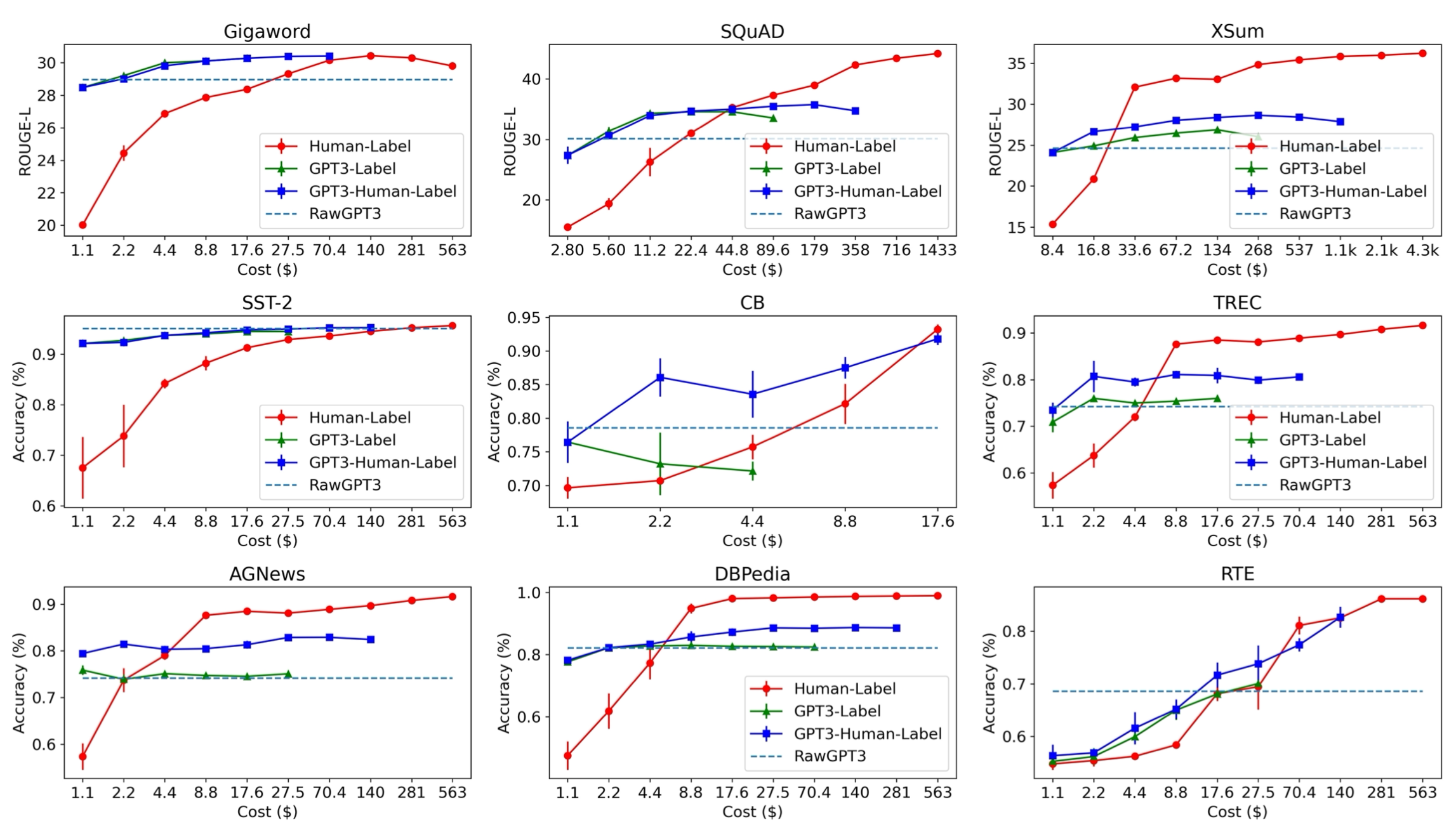
Wang et al. (2021) investigated how to use GPT-3 as a weak annotator via few-shot prompting, reporting labeling costs that are 10x lower than human annotation. The paper argues that training with GPT-3-labeled data effectively performs self-training: Predictions on unlabeled examples impose entropy regularization on the model, discouraging high class overlap and thereby improving performance.

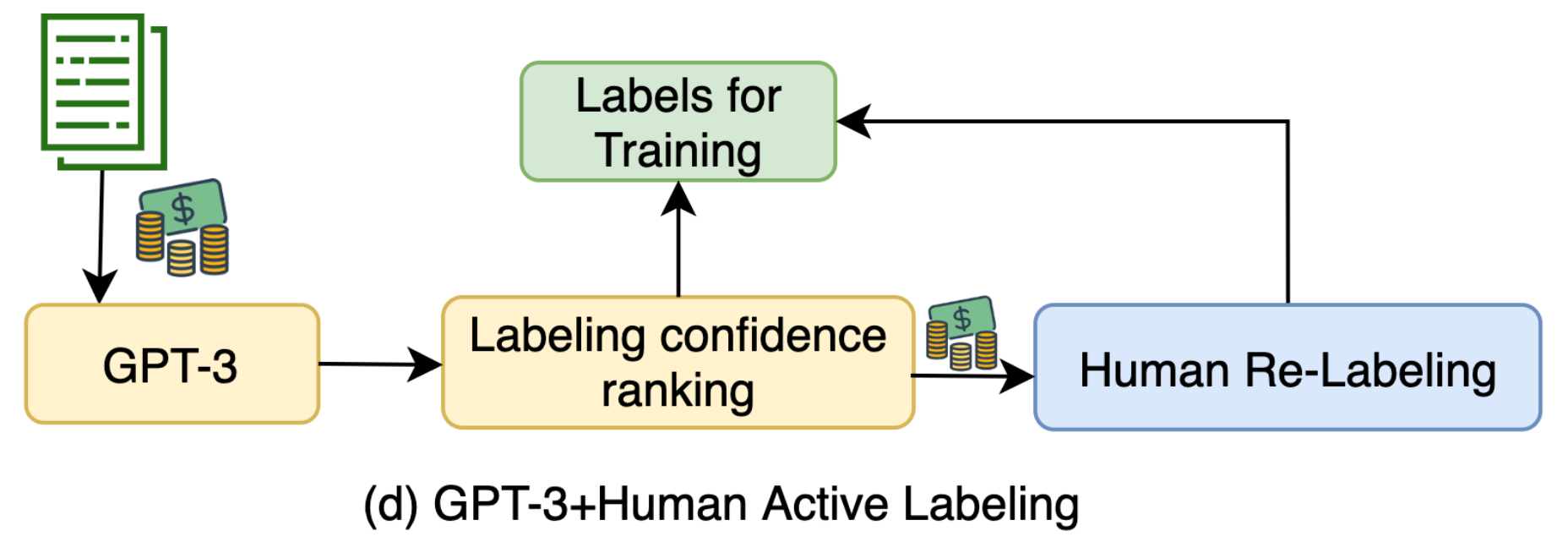
GPT-3-labeled samples selected via active learning (specifically those with the highest uncertainty) are routed to human annotators for re-labeling. Because the few-shot prompt includes only a small number of human-labeled examples, the human labeling cost remains bounded. Synthetic samples are ranked by predicted logits of label $y$, and those with the lowest scores are sent for relabeling.

GPT-3 labeling performs better in the low-cost regime, but it falls short of human labeling once sufficient resources are devoted to data collection. This motivates the following inequation, although the precise meaning of “a lot” and “noisy” depends on task specifics.

A lot of high-quality data > A lot of noisy data > A little high quality data.

Language Model as Data Generator

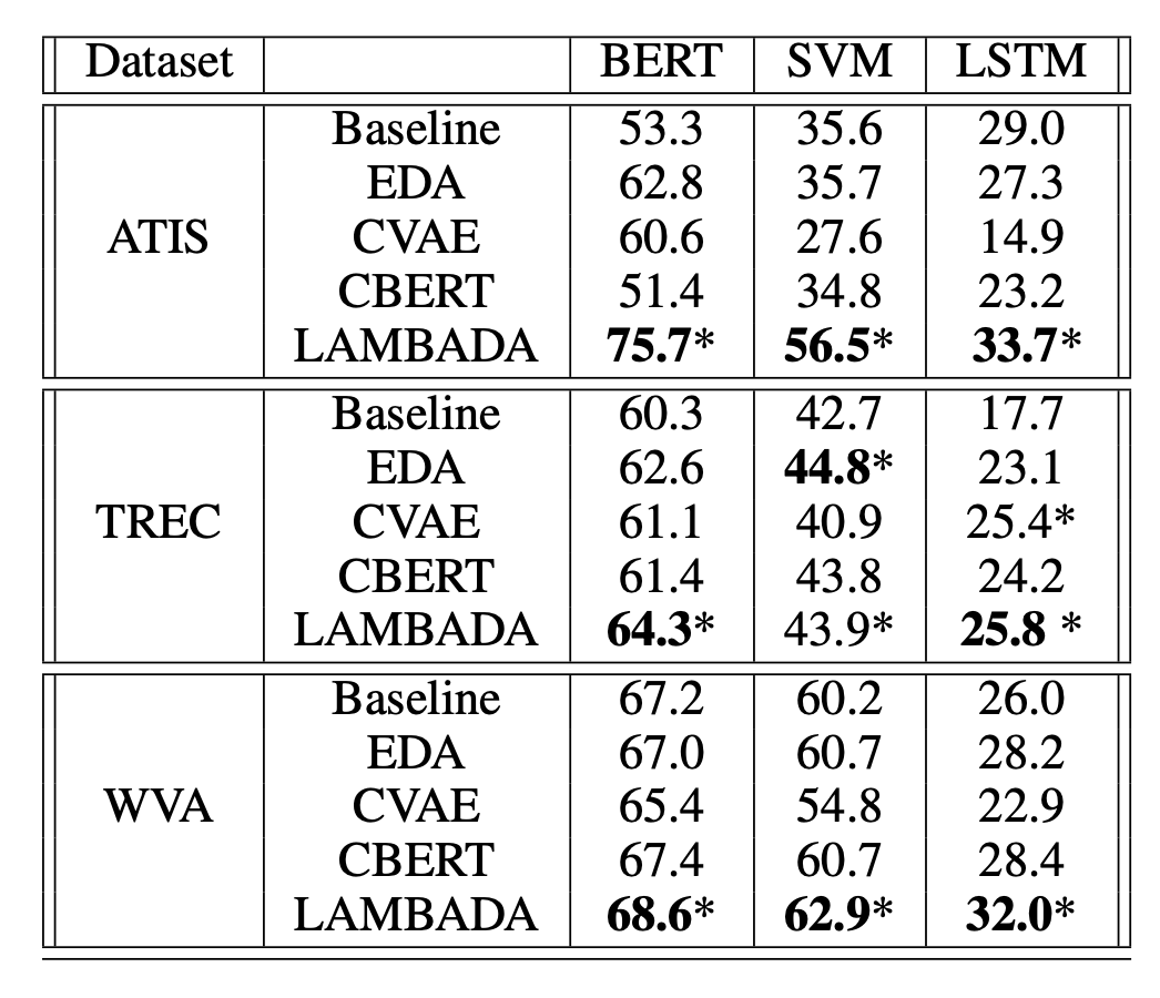
When sufficiently large training datasets are available for text classification, language models can be fine-tuned to synthesize additional label-conditioned training samples (Anaby-Tavor et al. 2019, Kumar et al. 2021).

Language-model-based data augmentation (LAMBADA; Anaby-Tavor et al. 2019) instantiates this idea, using a workflow that fine-tunes both a classifier and a generation model.

1. Train a baseline classifier on the available training set: $h = \mathcal{A}(\mathcal{D}_\text{train})$.
2. Separately from step 1, fine-tune a LM $\mathcal{M}$ on $\mathcal{D}_{\text{train}}$ to obtain $\mathcal{M}_{\text{tuned}}$.
3. Generate a labeled synthetic dataset $\mathcal{D}^*$ by sampling continuations of the sequence y[SEP] until EOS using $\mathcal{M}_\text{tuned}$.
4. Filter the synthesized dataset by:
   • (1) Checking whether the predicted label matches the intended label $h(x)=y$;
   • (2) Ranking samples by classifier probability and keeping only top-ranked examples. $\mathcal{D}_\text{syn} \subset \mathcal{D}^*$. They generate 10x more samples than needed for augmentation, and retain only the top 10% with the highest confidence scores.

The final classifier is trained on $\mathcal{D}_\text{syn} \cup \mathcal{D}_\text{train}$. This process can be iterated multiple times, but it is unclear whether gains would quickly saturate or whether repetition would introduce self-bias.

To streamline LAMBADA, we can remove the dependence on both a fine-tuned generation model and a reasonably large existing training set (that is, Step 2 above). Unsupervised data generation (UDG; Wang et al. 2021) uses few-shot prompting with a large pretrained language model to produce high-quality synthetic training data. In contrast to the approach above, where the LM predicts $y$ given $\mathbf{x}$, UDG instead generates inputs $\mathbf{x}$ conditioned on labels $y$. A task-specific model is then trained on the resulting synthetic dataset.

Schick & Schutze (2021) proposed a related approach for NLI rather than classification, prompting a PLM with task instructions to write sentence pairs that are similar or different.

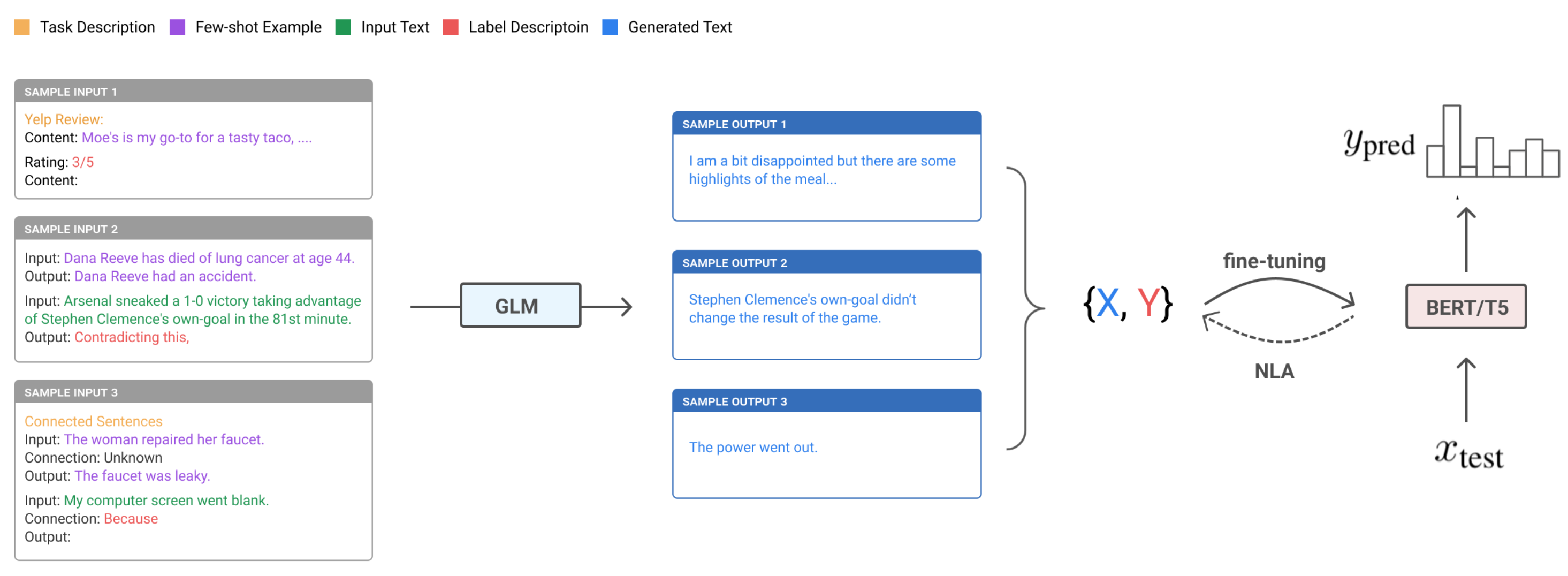
UDG few-shot prompts include a small set of unlabeled examples together with a task-specific natural-language description of the target label. Since some generated examples are noisy, the authors introduce noisy label annealing (NLA) to remove potentially misaligned samples during training. NLA progressively suppresses noisy training signals over time, specifically when the model disagrees with its pseudo-label with high confidence. At training step $t$, a sample $(\mathbf{x}_i, \hat{y}_i)$ is treated as noisy and removed if:

• The model’s predicted probability exceeds a threshold $p(\bar{y}_i \vert \mathbf{x}_i) > \mu_t$ where $\bar{y}_i = \arg\max_y p(y \vert \mathbf{x}_i)$;
• And the predicted label differs from the synthetic label, $\bar{y}_i \neq \hat{y}_i$.

Note that the threshold $\mu_t$ is time-varying: it starts at 0.9 and is gradually annealed toward $1/\text{num_of_classes}$ over time.

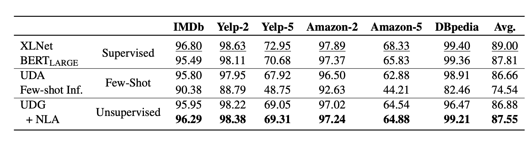
In their experiments, UDG improves substantially over few-shot inference, with NLA providing an additional boost. In several cases, results are even comparable to supervised fine-tuning.

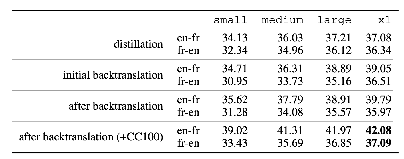
Han et al (2021) reported SOTA results on translation tasks using a combination of few-shot data generation, distillation, and back-translation. Their method consists of the following steps, assuming there is no access to paired translation data:

1. Zero-shot Generation. Use the zero-shot translation capability of a pretrained LM to generate translations for a small set of unlabeled sentences.
2. Few-shot Generation. Scale up the dataset by using these zero-shot translations as few-shot demonstrations to generate a much larger synthetic dataset.
3. Distillation. Fine-tune the model on the synthetic dataset. The translation task is expressed as a language modeling task [L1] <seq1> [[TRANSLATE]] [L2] <seq2>. given a pair <seq1, seq2> in two different languages. At test time, the LM is prompted with [L1] <seq> [[TRANSLATE]] [L2], and a candidate translation <sampledSeq> is extracted from the sampled completion.
4. Back-translation. Continue fine-tuning on a back-translation dataset with the sample order reversed, <sampledSeq, seq>.
5. Repeat steps 1 through 4 as needed.

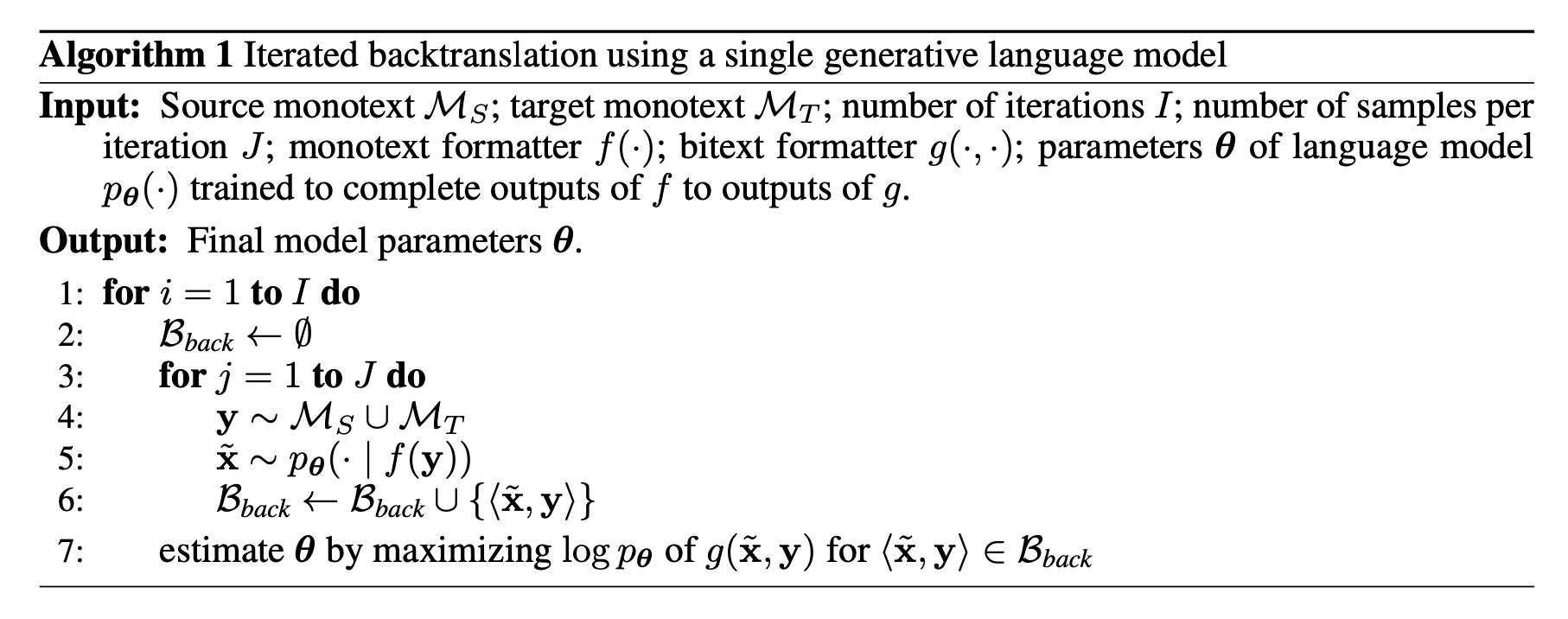
The effectiveness of this pipeline depends on having a strong pretrained LM to bootstrap the initial translation dataset. Iterative few-shot generation and distillation, together with back-translation, is an effective way to extract and refine translation capabilities from a pretrained LM, and then distill them into a new model.

How to Quantify Generated Data Quality?

Once data has been generated, via either augmentation or synthesis, how should we measure its quality in terms of its contribution to generalization? Gontijo-Lopes et al. (2020) proposed tracking two dimensions: affinity and diversity.

• Affinity is a model-sensitive measure of distribution shift, capturing how strongly an augmentation changes the training distribution relative to what a model learns.
  • Definition: The performance gap between evaluation on clean data and evaluation on augmented data, when the model is trained on clean data.
  • For comparison, KL divergence can also quantify distribution shift, but it does not incorporate model performance.
• Diversity measures augmentation complexity, representing how complex the augmented data is relative to the model and training procedure.
  • Definition: The final training loss of a model trained using a given augmentation.
  • Another possible diversity metric is the entropy of the transformed data.
  • A third possible diversity metric is the training time required for a model to reach a specified training-accuracy threshold.
  • All three metrics above are correlated.

Final model quality depends on both metrics being sufficiently high.

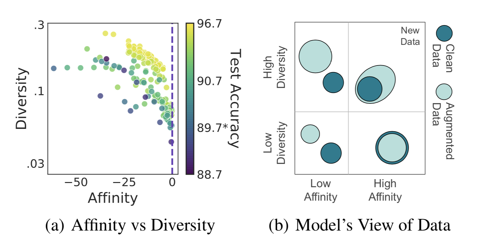
Many quantitative measures of relevance and diversity exist, and they take different forms depending on whether a reference is available, for example, perplexity and BLEU for text, or inception score for images. I am not listing specific quality metrics here, as the list would be extensive.

Training with Noisy Data

Collecting large amounts of noisy data through model generation or augmentation is often convenient, but it is difficult to ensure that augmented or generated samples are perfectly accurate. Since deep neural networks can readily overfit noisy labels and “memotize” corrupted labels, it is helpful to apply methods for learning with noisy labels (noise-robust training) when training on generated data, in order to stabilize and optimize performance. For a more comprehensive review of related work, see the survey paper (Song et al. 2021) on learning from noisy labels.

Regularization and Robust Architecture

In general, anti-overfitting mechanisms should improve robustness when training with moderately noisy data, including weight decay, dropout, and batch normalization. In fact, high-quality augmentation (that is, altering only non-essential attributes) can also be viewed as a form of regularization.

An alternative direction is to add a dedicated noisy adaptation layer to the network to approximate the unknown label-corruption projection (Sukhbaatar et al. 2015, Goldberger & Ben-Reuven, 2017).

Sukhbaatar et al. (2015) introduced an additional linear layer $Q$ in the network to adapt predictions so they align with the noisy label distribution. The noise matrix $Q$ is initialized as the identity function and held fixed, while only the base-model parameters are updated. After some training, $Q$ is also updated and is expected to capture dataset noise. The noise matrix is trained with regularization to encourage it to match the noise distribution while keeping the base model’s predictions accurate for the true labels.

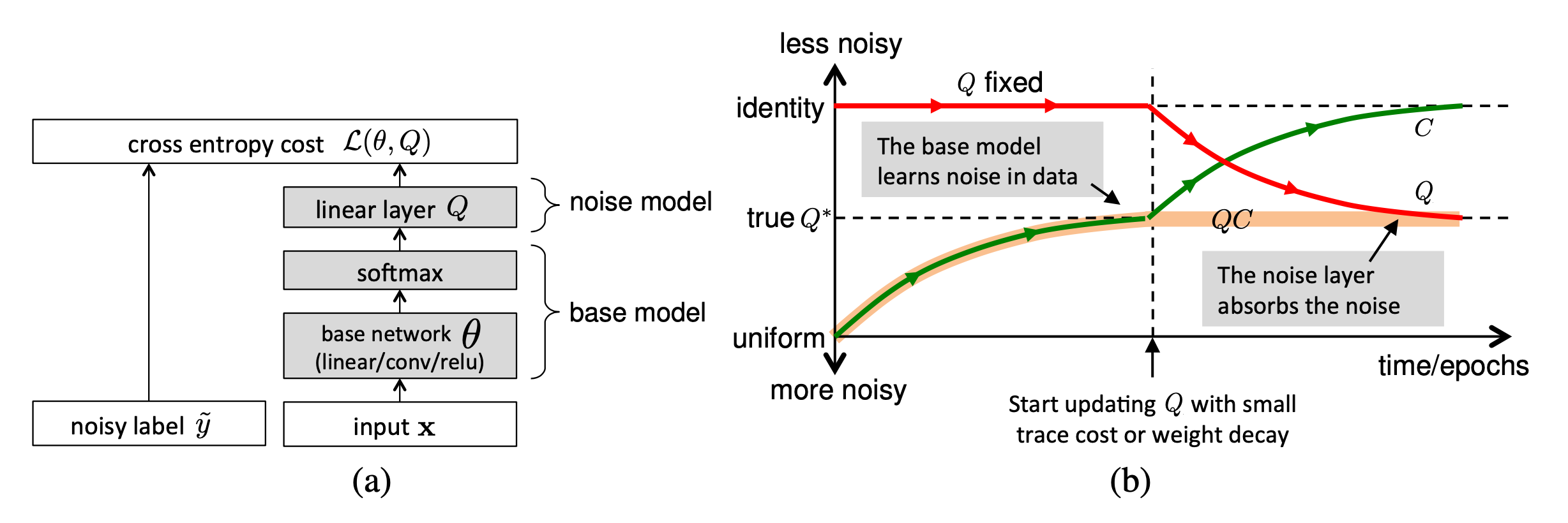
However, it is difficult to ensure that a noise-matrix layer captures only the noise-transition distribution, and learning it is not trivial. Goldberger & Ben-Reuven (2017)) proposed adding an additional softmax layer end-to-end with the base model and applying the EM algorithm, treating the correct labels as a latent random variable and modeling the noise process as a communication channel with unknown parameters.

Robust Learning Objective

In addition to the widely used cross-entropy loss, several alternative learning objectives have been shown to be more robust in the presence of noisy labels.

For instance, MAE (mean absolute error) is more robust to noisy labels than CCE (categorical cross entropy) because it assigns equal influence to every sample (Ghosh et al. 2017). However, because MAE does not provide differentiated weighting across training samples, it can require substantially longer training time. To address the tradeoff between MAE and CCE, Zhang & Sabuncu (2018) introduced generalized cross entropy (GCE), which generalizes the CCE loss to improve robustness to noisy data.

To combine the noise robustness of MAE with the implicit weighting behavior of CCE, GCE uses the negative Box-Cox transformation as its loss function:

$ \mathcal{L}_q(f(\mathbf{x}_i, y_i = j)) = \frac{1 - f^{(j)}(\mathbf{x}_i)^q}{q} $

where $f^{(j)}$ denotes the $j$-th element of $f(.)$ and $q \in (0, 1]$. $\mathcal{L}_q$ is equivalent to CCE when $q \to 0$, and it becomes MAE when $q=1$. Empirical results indicate that there exists a threshold value of $q$ under which overfitting does not occur, and that this threshold should be higher as the data become noisier.

Given true and predicted labels, $y_i, \hat{y}_i \in \{0, 1\}$ and let $u_i=y_i \cdot \hat{y}_i$, the zero-one loss, $\mathcal{L}_{01}(\mathbf{u}) = \sum_{i=1}^n \mathbb{1}[u_i < 0]$, is another learning objective that has been shown to be robust to noisy data. Minimizing empirical risk under the zero-one loss is shown to be equivalent to minimizing the empirical adversarial (worst-case) risk (Hu et al 2018). Because the worst-case risk upper-bounds the classification risk under the clean data distribution, reducing the worst-case risk can decrease the true risk, which makes the zero-one loss particularly robust. However, the zero-one loss is non-differentiable, so it cannot be optimized directly. A common workaround is to minimize an upper bound approximation of the zero-one loss instead.

The hinge loss, $\mathcal{L}_\text{hinge}(\mathbf{u}) = \sum_{i=1}^n \max(0, 1 - u_i)$, provides a coarse upper bound on the zero-one loss. Lyu & Tsang (2020) proposed a curriculum loss (CL), which yields a tighter upper bound than conventional surrogate losses such as the hinge loss, $\mathcal{L}_\text{01}(\mathbf{u}) \leq \mathcal{L}_\text{CL}(\mathbf{u}) \leq \mathcal{L}_\text{hinge}(\mathbf{u})$.

$ \mathcal{L}_\text{CL}(\mathbf{u}) = \min_{\mathbf{w}\in\{0,1\}^n}\max(\sum_{i=1}^n w_i \ell(u_i), n - \sum_{i=1}^n w_i + \sum_{i=1}^n\mathbb{1}[u_i < 0]) $

where $\ell(u_i)$ is a base surrogate loss for the zero-one loss (e.g. hinge loss), and the optimal weighting variable $\mathbf{w}$ is learned.

Given a label corruption rate $\rho$, the noise pruned curriculum loss (NPCL) is derived from the intuition that an ideal model should correctly classify $n(1-\rho)$ samples with clean labels, while misclassifying $n\rho$ corrupted labels. If $\rho$ is available as a known prior, then the number of samples to prune (those with the largest losses) is also known. Assuming $\ell(u_1) \leq \dots \leq \ell(u_n)$, then $u_{n(1-\rho)+1} = \dots = u_n =0$, and the NPCL below corresponds to the basic CL computed using only $n(1-\rho)$ samples:

$ \text{NPCL}(\mathbf{u}) = \min_{\mathbf{w}\in\{0,1\}^{n(1-\rho)}} \max(\sum_{i=1}^{n(1-\rho)} w_i \ell(u_i), n(1-\rho) - \sum_{i=1}^{n(1-\rho)} w_i) $

On CIFAR-10, NPCL is comparable to GCE and performs better as the noise rate increases.

Label Correction

When it is known that some labels are incorrect, noise-robust training can explicitly incorporate label correction.

One approach estimates a noise transition matrix and uses it to correct either the forward or backward loss, an approach known as F-correction (Patrini et al. 2017). First, assume there are $k$ classes, the noise transition matrix $C \in [0, 1]^{k\times k}$ is observable, and the label-flipping probability depends only on the label (not on the input), which corresponds to random classification noise (RCN). Let $\tilde{y}$ denote a corrupted label. Each entry of $C$ represents the probability that one label flips to another¹:

$ C_{ij} = p(\tilde{y}= j \vert y =i, \mathbf{x}) \approx p(\tilde{y}= j \vert y =i) $

With this, we can apply a forward label-correction procedure to incorporate prior knowledge from the noisy transition matrix into the model prediction.

$ \begin{aligned} \mathcal{L}(\hat{p}(\tilde{y}\vert\mathbf{x}), y) &= - \log \hat{p}(\tilde{y}=i\vert\mathbf{x}) \\ &= - \log \sum_{j=1}^k p(\tilde{y}=i\vert y=j) \hat{p}(y=j\vert\mathbf{x}) \\ &= - \log \sum_{j=1}^k C_{ji} \hat{p}(y=j\vert\mathbf{x}) \end{aligned} $

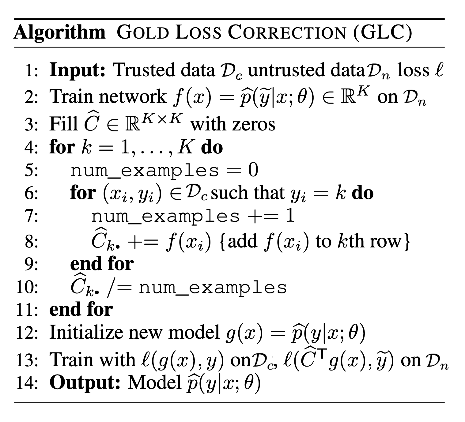
In matrix form, we have $\mathcal{L}(\hat{p}(y \vert \mathbf{x})) = - \log C^\top \hat{p}(y \vert \mathbf{x})$. In practice, however, the noise transition matrix is often unknown. If a clean dataset is available, the noise matrix $C$ can be estimated (Hendrycks et al. 2018) by computing a confusion matrix on clean data. Let a clean trusted dataset be denoted as $\mathcal{D}_c$ and a noisy dataset as $\mathcal{D}_n$.

$ \hat{C}_{ij} = \frac{1}{\vert \mathcal{A}_i\vert} \sum_{\mathbf{x} \in \mathcal{A}_i} \hat{p}(\tilde{y}=j \vert y=i, \mathbf{x}) \approx p(\tilde{y}=j \vert y=i) $

where $\mathcal{A}_i$ is a subset of data points from $\mathcal{D}_c$ with label $i$.

Let $f(x) = \hat{p}(\tilde{y} \vert \mathbf{x}; \theta)$; this model should be trained with $\mathcal{L}(f(\mathbf{x}), y)$ on clean data $\mathcal{D}_c$ and with $\mathcal{L}(\hat{C}^\top f(\mathbf{x}), \hat{y})$ on noisy data $\mathcal{D}_n$.

If the trusted training dataset $\mathcal{D}_c$ becomes sufficiently large, a neural network can be trained solely on clean data, and its knowledge can then be distilled into the primary model (that is, the final model used for test-time predictions) using corrected pseudo labels (Li et al. 2017). The primary model is trained on the full dataset, $\mathcal{D} = \mathcal{D}_c \cup \mathcal{D}_n$. Optionally, if “side” information describing label relations in a knowledge graph is available, it can be incorporated into distillation to improve the robustness of predictions when the network is trained with limited clean data.

Label-correction distillation proceeds as follows:

1. Train an auxiliary model $f_c$ using the small clean dataset $\mathcal{D}_c$. This model provides a soft label for each sample $x_i$; $s_i = \delta(f_c(\mathbf{x}_i)/T)$ is the sigmoid activation with temperature $T$.
2. Because the clean dataset is small, $f_c$ is likely to overfit. Li et al. (2017) therefore leverage a knowledge graph $\mathcal{G}$ that encodes relationships in the label space and propagate predictions across related labels. The resulting soft label is denoted as $\hat{s}_i = \mathcal{G}(s_i)$.
3. Train the primary model $f$ to imitate predictions from $f_c$:

$ \mathcal{L}(y_i, f(\mathbf{x}_i)) = \text{CE}(\underbrace{\lambda y_i + (1 - \lambda) \hat{s}_i}_\text{pseudo label}, f(\mathbf{x}_i)) $

Sample Reweighting and Selection

Some training examples are more likely than others to carry inaccurate labels. Estimating this likelihood provides guidance on which samples should receive lower or higher weight in the loss. However, when accounting for both class imbalance and noisy labels, the preferred bias can be contradictory: larger-loss samples may help rebalance the label distribution, while smaller-loss samples are often preferred to reduce the impact of label noise. Some work (Ren et al. 2018) therefore argues that, to learn general forms of training-data bias, it is necessary to have a small unbiased validation set to guide training. The reweighting methods in this section all assume access to a small trusted set of clean data.

For a binary classification task under random classification noise, $y, \hat{y} \in \{-1, +1\}$, the label-flipping probabilities, $\rho_{-1}, \rho_{+1} \in [0, 0.5)$, are defined as:

$ \rho_{-1} = P(\tilde{y} = +1 \vert y=-1)\quad\rho_{+1} = P(\tilde{y}=-1 \vert y =+1) $

Liu & Tao (2015) applies importance reweighting to adjust the weighted distribution of observed $\hat{y}$ so that it matches the distribution of the unobservable $y$. Let $\mathcal{D}$ be the true data distribution and $\mathcal{D}_\rho$ its corrupted counterpart.

$ \begin{aligned} \mathcal{L}_{\ell,\mathcal{D}}(f) &= \mathbb{E}_{(\mathbf{x},y)\sim \mathcal{D}}[\ell(f(\mathbf{x}), y)] \\ &= \mathbb{E}_{(\mathbf{x},\tilde{y})\sim \mathcal{D}_\rho} \Big[ \frac{P_\mathcal{D}(\mathbf{x}, y=\tilde{y})}{P_{\mathcal{D}_\rho}(\mathbf{x}, \tilde{y})} \ell(f(\mathbf{x}), \tilde{y}) \Big] \\ &= \mathbb{E}_{(\mathbf{x},\tilde{y})\sim \mathcal{D}_\rho} \Big[ \frac{P_\mathcal{D}(y=\tilde{y} \vert \mathbf{x})}{P_{\mathcal{D}_\rho}(\tilde{y} \vert \mathbf{x})} \ell(f(\mathbf{x}), \tilde{y}) \Big] & \text{; because }P_\mathcal{D}(\mathbf{x})=P_{\mathcal{D}_\rho}(\mathbf{x}) \\ &= \mathbb{E}_{(\mathbf{x},\tilde{y})\sim \mathcal{D}_\rho} [ w(\mathbf{x}, \hat{y})\ell(f(\mathbf{x}), \tilde{y}) ] = \mathcal{L}_{w\ell,\mathcal{D}}(f) \end{aligned} $

Because:

$ \begin{aligned} P_{\mathcal{D}_\rho}(\tilde{y} \vert \mathbf{x}) &= P_\mathcal{D}(y = \tilde{y} \vert \mathbf{x}) P_{\mathcal{D}_\rho}(\tilde{y} \vert y=\tilde{y}) + P_\mathcal{D}(y = - \tilde{y} \vert \mathbf{x}) P_{\mathcal{D}_\rho}(\tilde{y} \vert y = - \tilde{y}) \\ &= P_\mathcal{D}(y = \tilde{y} \vert \mathbf{x}) (1 - P_{\mathcal{D}_\rho}(- \tilde{y} \vert y=\tilde{y})) + (1 - P_\mathcal{D}(y = \tilde{y} \vert \mathbf{x})) P_{\mathcal{D}_\rho}(\tilde{y} \vert y = - \tilde{y}) \\ &= P_\mathcal{D}(y = \tilde{y} \vert \mathbf{x}) (1 - \rho_{\tilde{y}}) + (1 - P_\mathcal{D}(y = \tilde{y} \vert \mathbf{x})) \rho_{-\tilde{y}} \\ &= P_\mathcal{D}(y = \tilde{y} \vert \mathbf{x})(1 - \rho_{\tilde{y}} - \rho_{-\tilde{y}}) + \rho_{-\tilde{y}} \end{aligned} $

the weight assigned to a noisy sample is:

$ w(x, \tilde{y}) = \frac{P_\mathcal{D}(y=\tilde{y} \vert \mathbf{x})}{P_{\mathcal{D}_\rho}(\tilde{y} \vert \mathbf{x})} = \frac{P_{\mathcal{D}_\rho}(\tilde{y} \vert \mathbf{x}) - \rho_{-\tilde{y}}}{(1-\rho_0-\rho_1) P_{\mathcal{D}_\rho}(\tilde{y} \vert \mathbf{x})} $

where $P_{\mathcal{D}_\rho}(\tilde{y} \vert \mathbf{x})$ can be estimated via simple logistic regression, although estimating the noise rates is more challenging. Naive cross-validation can work, but it is costly because quality depends on how many trusted labels are available. The paper first approximates upper bounds for the noise rates, $\rho_\tilde{y} \leq P_{\mathcal{D}_\rho}(- \tilde{y} \vert \mathbf{x})$, and then applies a mild assumption to estimate them efficiently, $\hat{\rho}_{\tilde{y}} = \min_{\mathbf{x} \in {\mathbf{x}_1, \dots, \mathbf{x}_n}} \hat{P}_{\mathcal{D}_\rho}(- \tilde{y} \vert \mathbf{x})$. In experiments, the benefit of importance reweighting varies by dataset and is generally more pronounced when noise rates are high.

Sample-reweighting schemes can also be learned using a separate network. Learning to reweight (L2R; Ren et al. 2018) is a meta-learning method that directly optimizes weights to maximize validation performance on a known clean dataset. Each example is assigned a weight based on its gradient direction. The weighted loss to minimize, $\theta^*(\mathbf{w})$, includes a set of training weights $\{w_i\}_{i=1}^n$ treated as unknown hyperparameters. These per-sample training weights $w_i$ are learned by minimizing the loss on an unbiased validation set, $\mathcal{D}_c = \{x^\text{valid}_j\}_{j=1}^m$.

$ \begin{aligned} \theta^{*}(\mathbf{w}) &= \arg\min_\theta \sum_{i=1}^n w_i f(x_i; \theta) \\ \text{where optimal }\mathbf{w}^{*} &= \arg\min_{\mathbf{w}, \mathbf{w} \geq \mathbf{0}} \frac{1}{m} \sum_{j=1}^m f(\mathbf{x}^\text{valid}_j; \theta^{*}(\mathbf{w})) \end{aligned} $

This learning procedure uses two nested optimization loops and is therefore computationally expensive, about 3x training time.

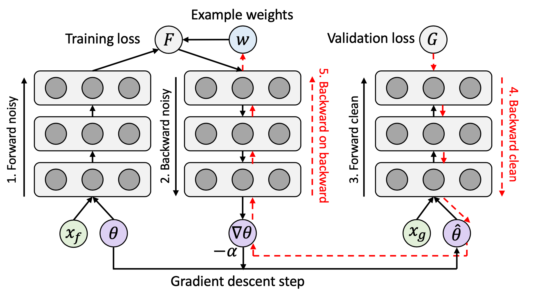
Experiments were conducted on: (1) a two-class MNIST setup to evaluate L2R robustness under class imbalance, and (2) CIFAR-10 with noisy labels. At the time, L2R was shown to outperform other baseline methods on both tasks.

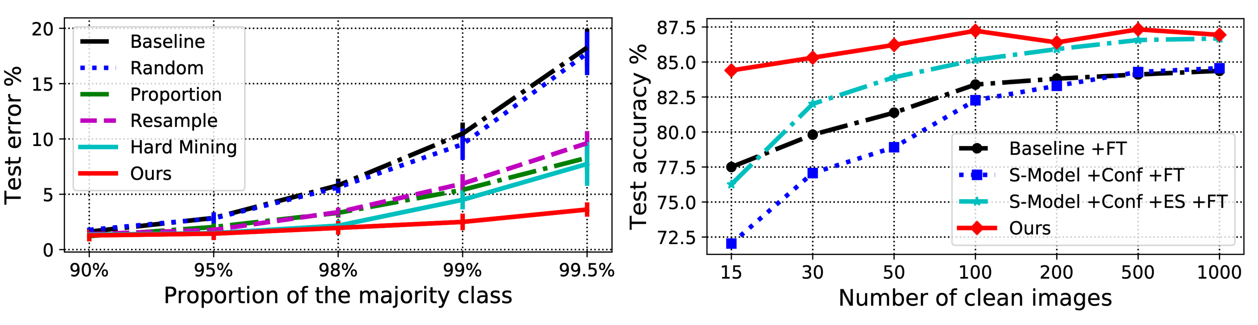
MentorNet (Jiang et al. 2018) uses a teacher-student curriculum-learning framework to weight data. It combines two networks, a mentor and a student. The mentor network provides a data-driven curriculum (that is, a sample-weighting scheme) that encourages the student to focus on samples that are likely to have correct labels.

Let $g_\psi$ be the MentorNet parameterized by $\psi$, $f_\theta$ be the StudentNet parametrized by $\theta$, and $G$ be a predefined curriculum parameterized by $\lambda$. Given training data $\mathcal{D} = \{(\mathbf{x}_i, y_i)\}_{i=1}^n$ for a $k$-class classification task, MentorNet predicts a time-varying latent weight variable $\mathbf{w} \in [0, 1]^{n \times k}$ to guide StudentNet learning, using an intermediate feature produced by StudentNet $f$, $\mathbf{z}_i = \phi_{f_\theta}(\mathbf{x}_i, y_i)$:

$ g_{\psi^{*}}(\mathbf{z}_i) = \arg\min_{w_i \in [0,1]} \mathcal{L}(\theta, \mathbf{w}), \forall i \in [1, n] $

StudentNet is trained to minimize the following objective:

$ \begin{aligned} \mathcal{L}(\theta, \mathbf{w}) &= \frac{1}{n}\sum_{i=1}^n \mathbf{w}_i^\top \ell(y_i, f_\theta(\mathbf{x}_i)) + G_\lambda(\mathbf{w}) + \alpha |\theta|^2_2 \\ &= \frac{1}{n}\sum_{i=1}^n g_\psi(\mathbf{z}_i)^\top \ell_i + G_\lambda(\mathbf{w}) + \alpha |\theta|^2_2 & \text{; Let }\ell_i = \ell(y_i, f_\theta(\mathbf{x}_i)) \\ \end{aligned} $

The mentor network $g_\psi$ is trained using cross entropy on input $(\phi_{f_\theta}(\mathbf{x}_i, y_i), w^{*}_i)$, where $v^*_i=1$ if $y_i$ is known to be a correct label, and 0 otherwise. MentorNet does not require a complex architecture; in the paper, an LSTM layer is used to capture time-varying prediction variance.

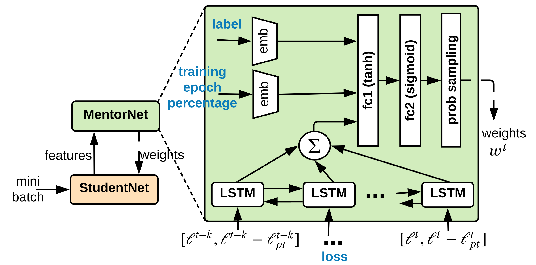
Unlike MentorNet, where one network explicitly learns a weighting scheme and curriculum for the other, Co-teaching (Han et al. 2018) trains two neural networks, $f_1$ and $f_2$, simultaneously and has them teach each other by selectively exchanging training data. Co-teaching consists of three steps:

1. Each network performs a forward pass on the current mini-batch and selects samples that are likely to have clean labels.
2. The two networks exchange their selected sample sets and decide which mini-batch samples to use for training. Small-loss instances are selected because they are more likely to be associated with correct labels. The fraction of the mini-batch retained is controlled by a time-dependent function $R(T)$. The value of $R(T)$ decreases over time because, as training continues, networks are more prone to overfit and memorize noisy labels; accordingly, a smaller sampling fraction is used to maintain high-quality selected data.
3. Each network updates its parameters via backpropagation using the samples selected by its peer.

In their experiments, co-teaching outperforms F-correction when noise rates are high or when the corruption transition matrix is not symmetric.

Citation

Cited as:

Weng, Lilian. (Apr 2022). Learning with not enough data part 3: data generation. Lil’Log. https://lilianweng.github.io/posts/2022-04-15-data-gen/.

Or

@article{weng2022datagen,
  title   = "Learning with not Enough Data Part 3: Data Generation",
  author  = "Weng, Lilian",
  journal = "Lil'Log",
  year    = "2022",
  month   = "Apr",
  url     = "https://lilianweng.github.io/posts/2022-04-15-data-gen/"
}

Reference

[1] Zhang et al. “Adversarial AutoAgument” ICLR 2020.

[2] Kumar et al. “Data Augmentation using Pre-trained Transformer Models.” AACL 2020 Workshop.

[3] Anaby-Tavor et al. “Not enough data? Deep learning to rescue!” AAAI 2020.

[4] Wang et al. “Want To Reduce Labeling Cost? GPT-3 Can Help.” EMNLP 2021.

[5] Wang et al. “Towards Zero-Label Language Learning.” arXiv preprint arXiv:2109.09193 (2021).

[6] Schick & Schutze. Generating Datasets with Pretrained Language Models." EMNLP 2021.

[7] Han et al. “Unsupervised Neural Machine Translation with Generative Language Models Only.” arXiv preprint arXiv:2110.05448 (2021).

[8] Guo et al. “Augmenting data with mixup for sentence classification: An empirical study.” arXiv preprint arXiv:1905.08941 (2019).

[9] Ekin D. Cubuk et al. “AutoAugment: Learning augmentation policies from data.” arXiv preprint arXiv:1805.09501 (2018).

[10] Daniel Ho et al. “Population Based Augmentation: Efficient Learning of Augmentation Policy Schedules.” ICML 2019.

[11] Cubuk & Zoph et al. “RandAugment: Practical automated data augmentation with a reduced search space.” arXiv preprint arXiv:1909.13719 (2019).

[12] Zhang et al. “mixup: Beyond Empirical Risk Minimization.” ICLR 2017.

[13] Yun et al. “CutMix: Regularization Strategy to Train Strong Classifiers with Localizable Features.” ICCV 2019.

[14] Kalantidis et al. “Mixing of Contrastive Hard Negatives” NeuriPS 2020.

[15] Wei & Zou. “EDA: Easy data augmentation techniques for boosting performance on text classification tasks.” EMNLP-IJCNLP 2019.

[16] Kobayashi. “Contextual Augmentation: Data Augmentation by Words with Paradigmatic Relations.” NAACL 2018

[17] Fang et al. “CERT: Contrastive self-supervised learning for language understanding.” arXiv preprint arXiv:2005.12766 (2020).

[18] Gao et al. “SimCSE: Simple Contrastive Learning of Sentence Embeddings.” arXiv preprint arXiv:2104.08821 (2020). [code]

[19] Shen et al. “A Simple but Tough-to-Beat Data Augmentation Approach for Natural Language Understanding and Generation.” arXiv preprint arXiv:2009.13818 (2020) [code]

[20] Wang & van den Oord. “Multi-Format Contrastive Learning of Audio Representations.” NeuriPS Workshop 2020.

[21] Wu et al. “Conditional BERT Contextual Augmentation” arXiv preprint arXiv:1812.06705 (2018).

[22 Zhu et al. “FreeLB: Enhanced Adversarial Training for Natural Language Understanding.” ICLR 2020.

[23] Affinity and Diversity: Quantifying Mechanisms of Data Augmentation Gontijo-Lopes et al. 2020 (https://arxiv.org/abs/2002.08973)

[24] Song et al. “Learning from Noisy Labels with Deep Neural Networks: A Survey.” TNNLS 2020.

[25] Zhang & Sabuncu. “Generalized cross entropy loss for training deep neural networks with noisy labels.” NeuriPS 2018.

[26] Goldberger & Ben-Reuven. “Training deep neural-networks using a noise adaptation layer.” ICLR 2017.

[27] Sukhbaatar et al. “Training convolutional networks with noisy labels.” ICLR Workshop 2015.

[28] Patrini et al. “Making Deep Neural Networks Robust to Label Noise: a Loss Correction Approach” CVPR 2017.

[29] Hendrycks et al. “Using trusted data to train deep networks on labels corrupted by severe noise.” NeuriPS 2018.

[30] Zhang & Sabuncu. “Generalized cross entropy loss for training deep neural networks with noisy labels.” NeuriPS 2018.

[31] Lyu & Tsang. “Curriculum loss: Robust learning and generalization against label corruption.” ICLR 2020.

[32] Han et al. “Co-teaching: Robust training of deep neural networks with extremely noisy labels.” NeuriPS 2018. (code)

[33] Ren et al. “Learning to reweight examples for robust deep learning.” ICML 2018.

[34] Jiang et al. “MentorNet: Learning data-driven curriculum for very deep neural networks on corrupted labels.” ICML 2018.

[35] Li et al. “Learning from noisy labels with distillation.” ICCV 2017.

[36] Liu & Tao. “Classification with noisy labels by importance reweighting.” TPAMI 2015.

[37] Ghosh, et al. “Robust loss functions under label noise for deep neural networks.” AAAI 2017.

[38] Hu et al. “Does Distributionally Robust Supervised Learning Give Robust Classifiers? “ ICML 2018.